

Independent Curves and Numerical Families
This guide covers GX-TXT Curve Digitalizer 0.9.8.10-dev-112, updated to patch P005. The control labels are given as they appear in the English interface.
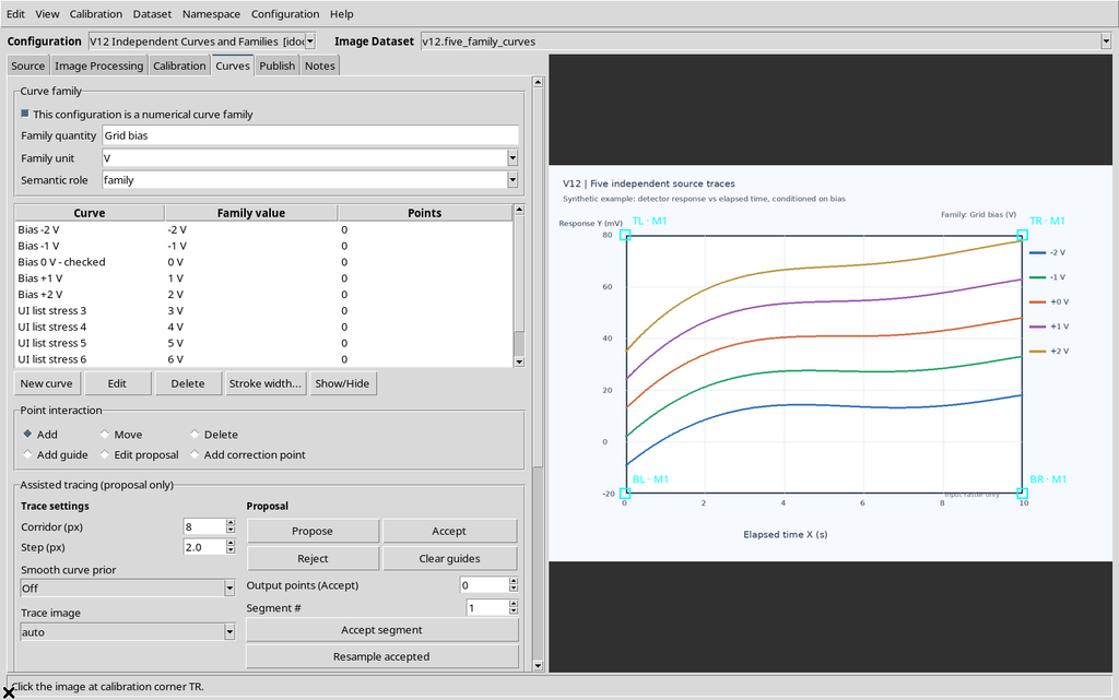
This chapter shows how to organize curves before digitizing points: creating and editing independent series, labels and identifiers, visibility, numerical families, scrolling, deletion and saving. The five colored traces are part of the source image, not numerical data already digitized.
1. A Graph with Five Source Traces
The example uses a single canonical Image Dataset with the image.raster contract: a synthetic 1280 × 900 pixel PNG. The image contains five detector response traces, corresponding to five bias voltages.
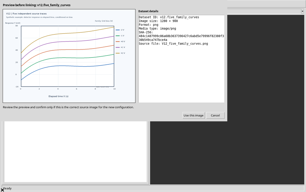
The figure was created for the tutorial, not acquired from an instrument. The raster curves have visual names and colors that are not automatically equivalent to the scientific objects of the Curves tab: these are created by the operator, separately.
2. The Scientific Axes Are Shared by the Curves of the Same Graph
In the Calibration panel, the physical axes Elapsed time, X=0–10 s, and Detector response, Y=−20–80 mV, were set, both linear. The calibration was acquired with the actual Set BL, Set BR, Set TL and Set TR buttons on the four corners of the plotted area.
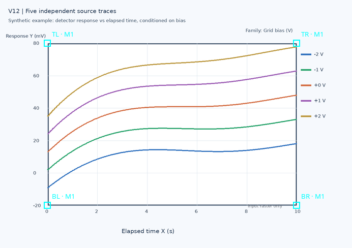
In this test all five future curves will share the same geometrically calibrated transformation. There is no need to invent five independent homographies for five lines drawn on the same axes.
The association with the different bias values belongs to the family metadata, not to the four calibration corners.
3. The Curves Tab in an Empty Configuration
Opening Curves in the new configuration, there are the Curve family frame, the curve table, the New curve, Edit, Delete, Stroke width… and Show/Hide commands, as well as the controls for points and assisted proposals.
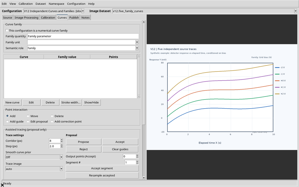
The initial table contains no scientific curves. The source, however, already shows five colored traces: their presence on screen does not prove that five curves exist in the Workspace.
This distinction between the original raster and the Series objects is fundamental for interpreting the future Dataset Preview correctly as well.
4. New curve: Label and Optional Properties
Pressing New curve opens the native dialog with the fields:
Curve label, Family parameter value (optional) and Family unit (optional).
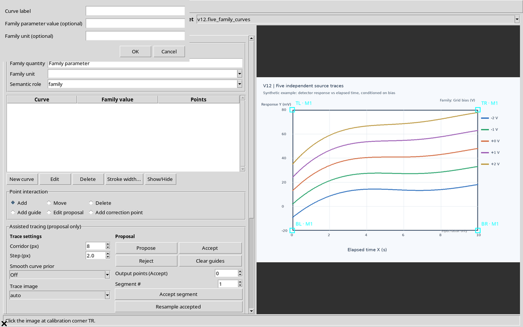
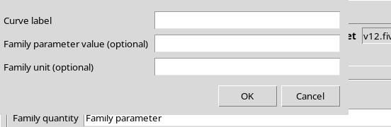
When the configuration is not a numerical family, it is legitimate to create independent curves leaving the last two fields empty. For example, two traces that represent different measurements and are not parameterized by the same quantity must not be artificially forced into a family.
5. The Curve label Field Is Required
OK was pressed with the curve name left empty. The GUI showed the error:
Curve label is required.
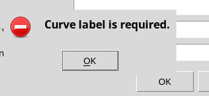
No curve without a label was created. Entering Reference blue with the two family fields empty and pressing OK, the viewer created a curve with a stable identifier and zero points.
The display name must not be used as the scientific key of the Dataset: the model keeps a separate identifier for each curve.
6. Two Independent Curves in Generic Mode
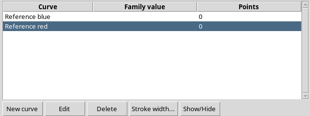
A second curve, Reference red, was added without a numerical parameter. Two rows appeared in the table with an empty Family value and Points = 0.
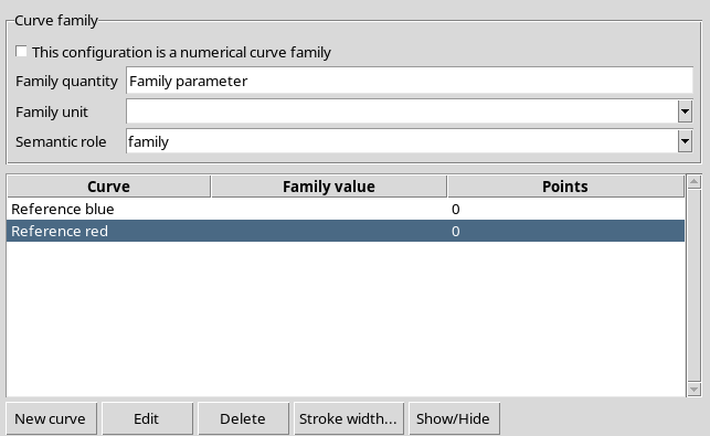
The publication contract of the generic configuration is table.generic. The presence of the two curves does not yet imply a publication: no X/Y points have been acquired.
The colors the Viewer assigns to curve objects must not be confused with those of the source pixels, especially before digitization.
7. Show/Hide: Changing Visibility Does Not Mean Changing the Source
With the second curve selected, Show/Hide was pressed. The table added the text (hidden) to the curve label.
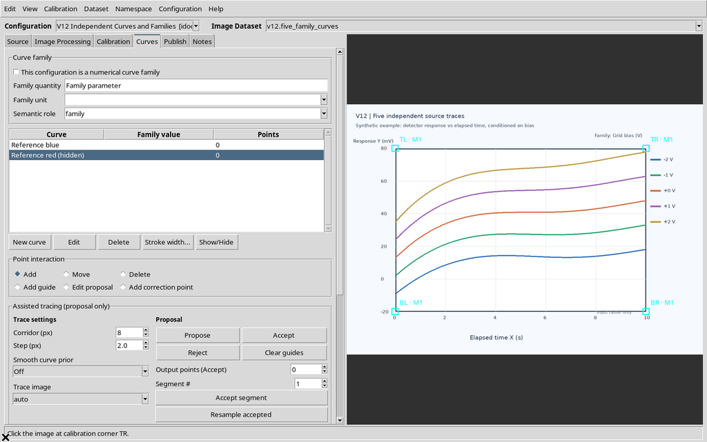
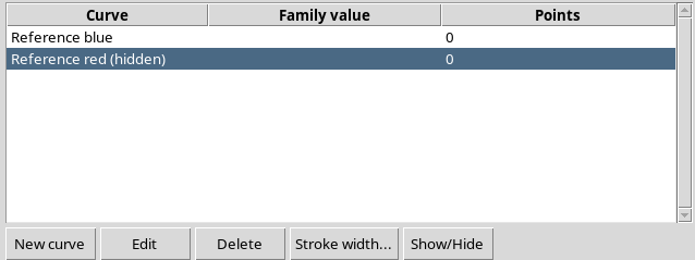
The viewer changed only the visible field of the selected curve. The scientific identifier, the number of points (still zero), the axes and the SHA-256 of the image stayed identical. The five colored lines contained in the PNG stayed visible because they are part of the original raster.
Pressing Show/Hide again, the curve became visible again. It was neither deleted nor duplicated.
8. When a Configuration Is a Numerical Family
The Curve family frame contains the This configuration is a numerical curve family checkbox, along with the Family quantity, Family unit and Semantic role fields.
For our example the following were used:
| Control | Value |
|---|---|
| This configuration is a numerical curve family | Enabled |
| Family quantity | Grid bias |
| Family unit | V |
| Semantic role | family |
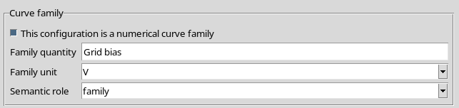
A numerical family makes sense when a common physical quantity parameterizes all the curves, such as grid voltage, temperature or concentration. It is not enough for the lines to be close together or to have different colors.
9. Enabling the Family Does Not Invent Missing Values
The family checkbox was enabled while there were still two curves with empty optional values. The GUI kept both rows, without automatically assigning bias numbers.
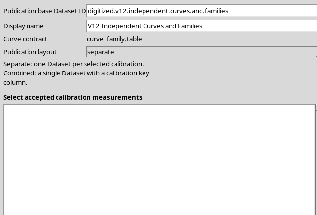
The proposed output switched to the curve_family.table contract, visible in the Publish tab.
This step changes the intended publishing mode and semantics, but does not automatically fulfil the scientific requirements. Curve Digitalizer requires finite numerical values and consistent units before publishing a family.
10. Edit curve: Assigning the Family Values
Selecting the first curve and pressing Edit, Curve label = Bias -2 V, Family parameter value = -2 and Family unit = V were set.
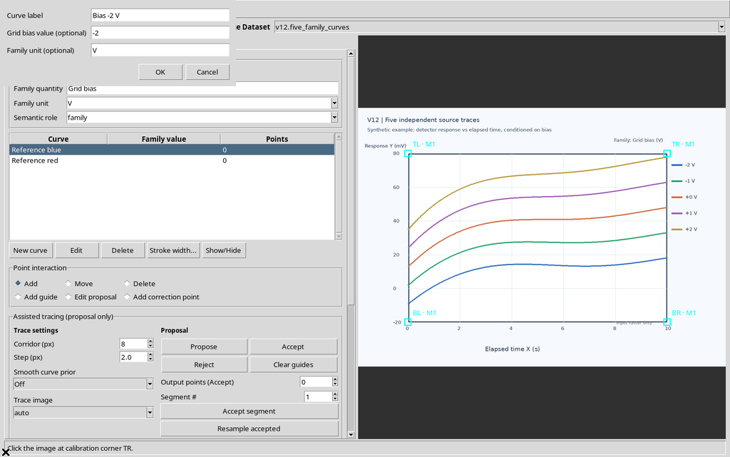
The second curve was modified in the same way to Bias -1 V, value -1, unit V.
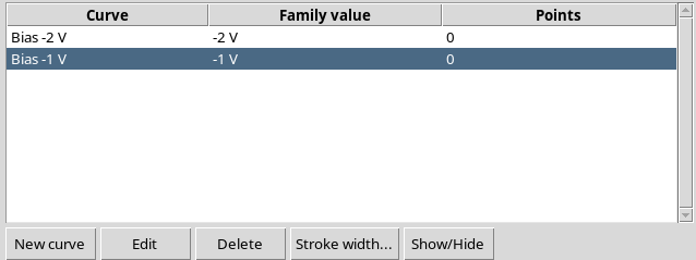
Comparing the Workspace before and after Edit confirmed that both curves keep the same identifiers. The names and family data changed, not the reference scientific curves or the source.
11. Completing the Five Curves
With New curve, three more series were created: Bias 0 V, Bias +1 V and Bias +2 V, each with the corresponding numerical value and the unit V.
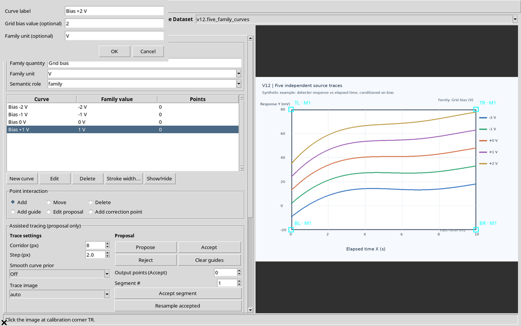
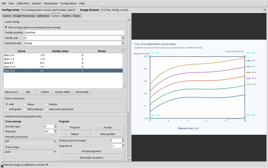
The result is a family of five Series objects, all distinct by ID and all still without points. The five traces visible in the image are available as a visual reference for the later digitization, but none has been converted automatically into X/Y data.
12. A Family Complete with Metadata
The final table of the Curves tab has the following rows:
| Curve label | Family value | Points |
|---|---|---|
| Bias -2 V | −2 V | 0 |
| Bias -1 V | −1 V | 0 |
| Bias 0 V | 0 V | 0 |
| Bias +1 V | +1 V | 0 |
| Bias +2 V | +2 V | 0 |
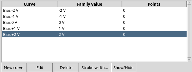
The viewer keeps these values inside the parameter metadata of each curve, in three distinct attributes: quantity name, value and unit. The group also has its own family definition with the enabled state and the semantic role.
A family value of 0 V is numerically valid: it must not be confused with a missing value.
13. Colored Trace and Scientific Curve Are Different Things
The source image shows five traces with different colors and a legend. The curve list shows five scientific objects with numerical bias values.
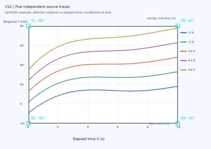
Their equal number was built intentionally for the tutorial, but it does not prove that each object is already associated with the pixels of the right line. This correspondence will be built by digitizing points on the correct curve in the following chapters.
Even a visible curve with Points = 0 does not automatically produce a vector line of data: the drawing still belongs to the source PNG.
14. The curve_family.table Contract Is Not an Already Published Dataset
The Curve contract field in the Publish tab shows curve_family.table when the family is enabled. In non-family mode, the contract shown is table.generic.
The intended contract describes how the data would be published if numerical curves were ready, with valid family parameters and admitted calibrations.
15. Disabling the Family Keeps the Curves and Their Values
After the five series were created, This configuration is a numerical curve family was disabled.
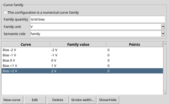
The mode became generic and the contract went back to table.generic.
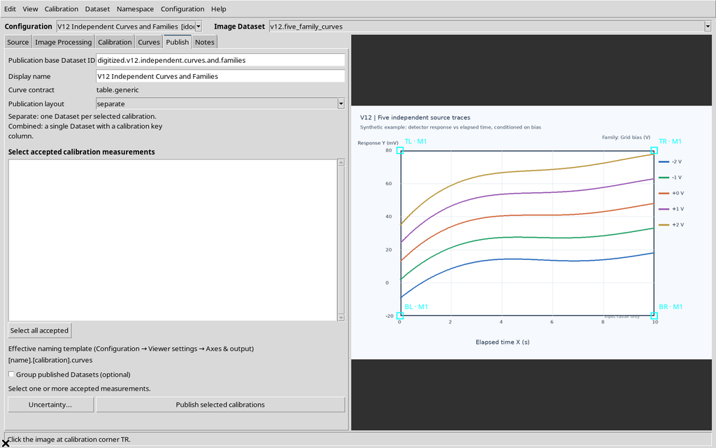
The five IDs, the five labels and the values −2, −1, 0, +1, +2 V stayed exactly as before. Disabling the family does not mean deleting the metadata of the individual curves, nor clearing the Series objects.
16. Re-enabling the Family Restores the Group Semantics
The family checkbox was then re-enabled in the same configuration, without recreating the curves.
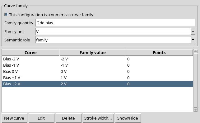
This option lets you correct the classification of a configuration; it must not be used to arbitrarily give heterogeneous series a common numerical meaning.
17. Cancel in Edit curve Does Not Save the Draft
On the Bias 0 V curve, Edit curve was opened and a deliberately wrong name, value and unit were entered temporarily, without confirming them.
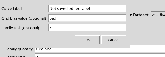
Pressing Cancel, the table and the Workspace keep the original values.
18. Changing Curve label Does Not Change the Curve ID
Opening Edit curve a second time, only the label was changed to Bias 0 V – checked, keeping the parameter 0 V.
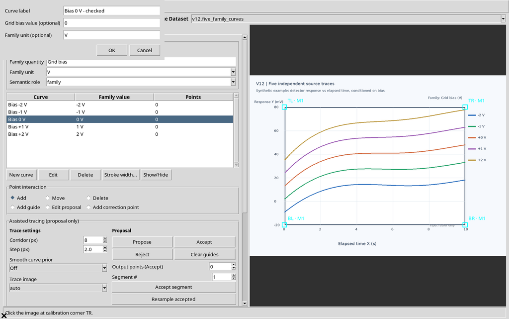
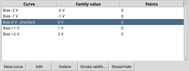
In the run for this guide the label was then set back to Bias 0 V, in agreement with the legend of the image.
19. Long Lists Have Their Own Scrolling
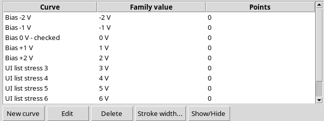
To show the list scrolling, six empty temporary curves were created, named UI list stress 3 through UI list stress 8. They serve only to make the list long enough to scroll; they do not correspond to other traces in the image.
The table thus has eleven rows: more than the nine that can be shown at once. These six temporary curves do not correspond to new traces in the image and are removed before the end of the chapter.
20. List Scrolling Is Independent of the Curves Page
The vertical control of the table was moved first to the beginning and then to the end of the list.
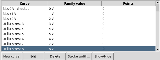
There are therefore two different scrollable areas: the curve list must not accidentally drag the whole control panel. Zooming the raster on the right is also a separate function.
21. Delete Requires Confirmation
Selecting the temporary curve UI list stress 8 and pressing Delete, the interface shows:
Delete curve ‘UI list stress 8’ and its 0 points?
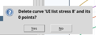
Choosing No keeps the list of eleven curves. Repeating the operation and choosing Yes, only that temporary curve is deleted.
This command is stronger than Show/Hide and Cancel: it actually removes the selected scientific object. In our example the message shows 0 points, so no numerical data were deleted.
22. Cleaning Up the Temporary Curves and Checking the IDs
The other five curves created for scrolling are removed with the Delete command and the corresponding native confirmation.
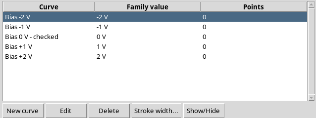
The Workspace went back to containing exactly the five initial curves.
23. Back to the Five Labels of the Graph
The temporarily renamed curve was set back to Bias 0 V. All five labels in the table now match the values of the legend in the raster, with the unit V.
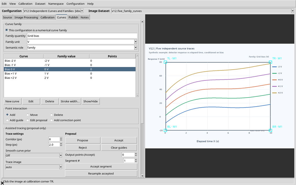
This correspondence is an organizational choice for the example, not an automatic scientific measurement. To turn the lines into data you still need to select the correct curve and enter its points with the tools available in the Viewer.
24. Accepted Calibration and Numerically Empty Series
The already complete calibration of the same image was classified accepted with the Accept button of the Calibration tab.
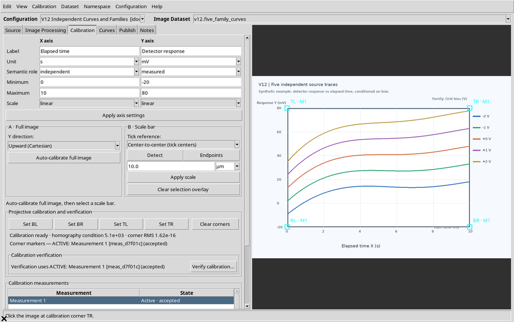
The result includes a group with one accepted calibration measurement and five parameterized series, but all with Points = 0. The accepted state of the calibration does not make the curves automatically ready for publishing.
This avoids a common confusion between approving the geometric transformation and accepting actually sampled curve data.
25. Publish: Observing the Contract Without Publishing
With the family enabled again, the Publish tab shows:
- Curve contract =
curve_family.table; - the Publication layout option with
separateandcombined; - one accepted calibration measurement among the eligible ones.
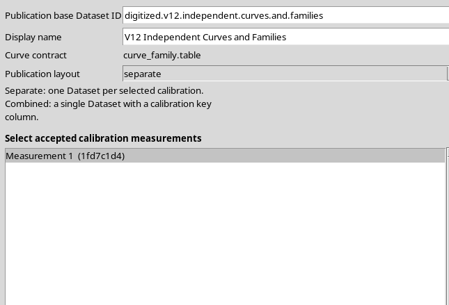
The two layout options were only observed. Publish selected calibrations was not pressed, because there are no numerical points.
A later publication of numerical families requires finite values and consistent family units. This example does not publish anything and shows no resulting numerical Datasets.
26. Save, Close and Reopen: Checking Persistence
The final configuration was saved from the Configuration → Save configuration menu, then the Viewer was closed normally and reopened from the Viewers → Digitalizer catalog, in the same synthetic Session.
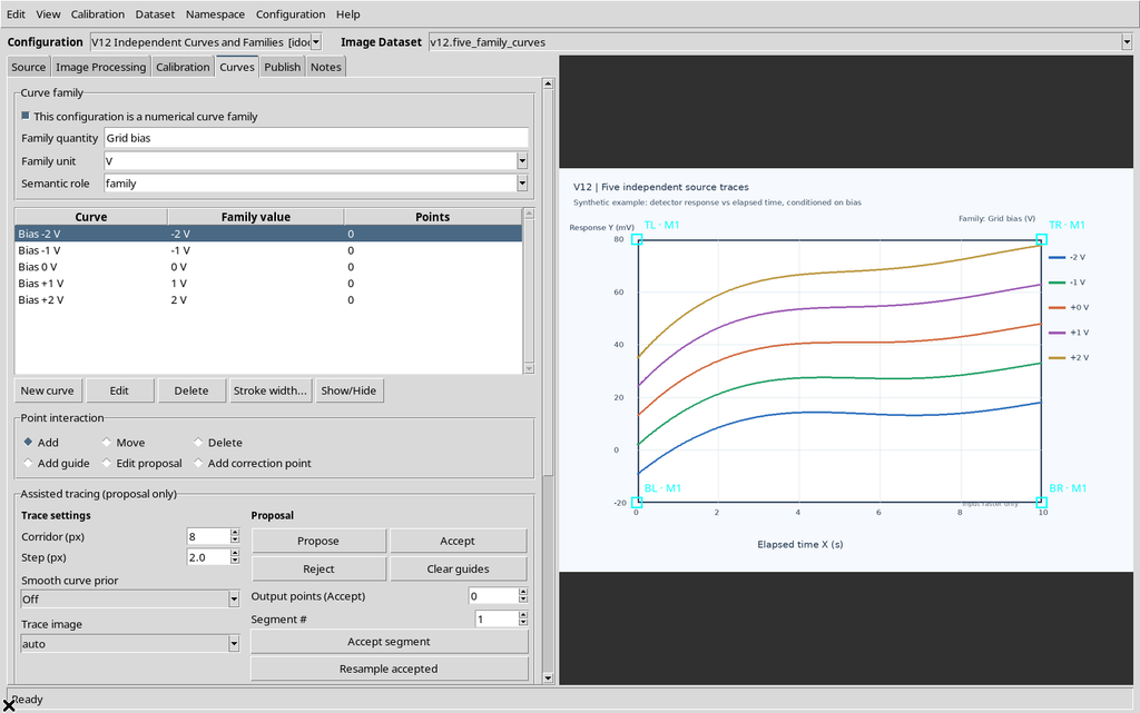
The framework returned the same five identifiers, names and family values, the same Grid bias / V / family definition, the unchanged canonical source, the physical X/Y axes, the accepted calibration and the four corners.
The six temporary curves did not reappear. The Viewer stayed consistent with what had actually been saved, with no changes to the raster.
27. Meaning of the Data and Limits of the Test
This guide verifies the structure of the curves and the classification of the family, not the sampling or the publication of numerical data.
The scientific Series objects have distinct IDs and family metadata, but hold zero points. Consequently, only the source Image Dataset remains in the Session Dataset Catalog. There is not yet a canonical table of digitized data to compare with the Dataset Preview, nor a Plot Dataset API v4 result.
The visibility state concerns the presentation of the series, not the source pixels. The family value is a numerical property that identifies a described experimental condition, not a measure of uncertainty or a new observation of the Y response.
28. Essential Operating Procedure
For independent curves, create the objects with New curve, enter a label and leave the family fields empty when there is no common numerical quantity.
For a scientific family, enable This configuration is a numerical curve family and set Family quantity, Family unit and Semantic role. For each curve, enter a numerical value and the consistent unit through New curve or Edit curve.
Use Show/Hide to change only the presentation and Delete only when you really want to remove the series, checking the confirmation. Before closing, save the configuration and check that the IDs and family values have been kept.