

Publishing Independent Curves and Numerical Families
A single image can contain several traces. The GX-TXT Curve Digitalizer lets you acquire them as independent scientific curves, each with its own identity, or as a numerical family, in which each curve is associated with a physical condition.
The two modes do not require the points to be digitized again. What changes is the structure of the published Dataset: independent curves use table.generic, a family uses curve_family.table. In both cases the grouping of points depends on the curve key, not on its visible label.
The example is a synthetic teaching raster, not an instrument experiment. The guide concerns a single accepted calibration and the separate publication layout. Handling several calibrations, the combined layout and advanced naming rules is covered separately.
1. A Source with Five Traces
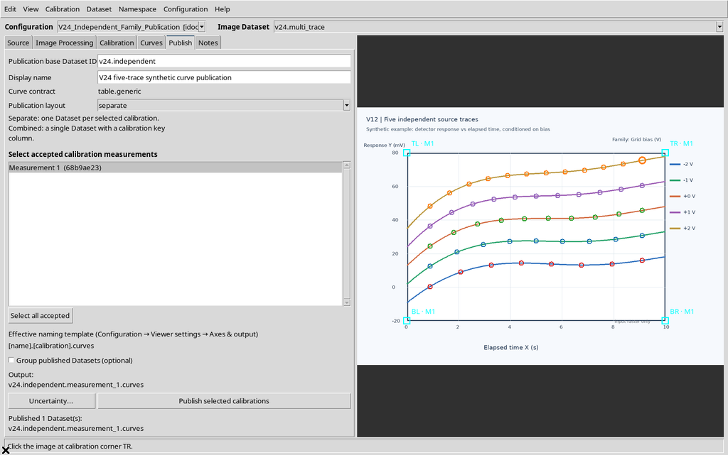
The original image shows five colored lines on a grid, with a legend that associates each line with a Grid bias condition between −2 and +2 V.
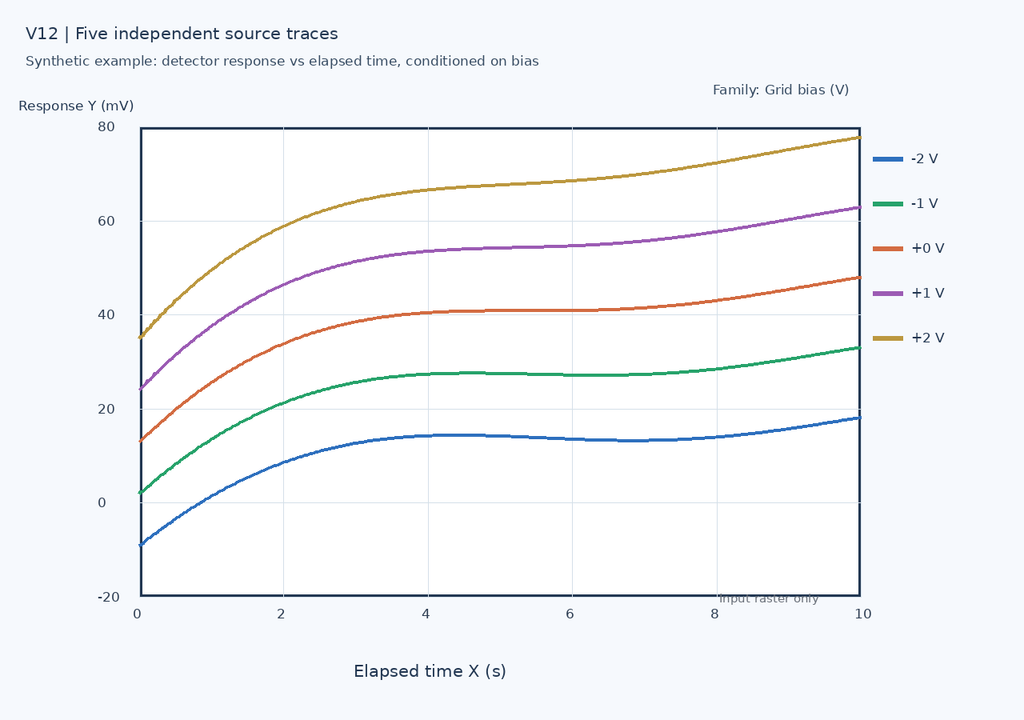
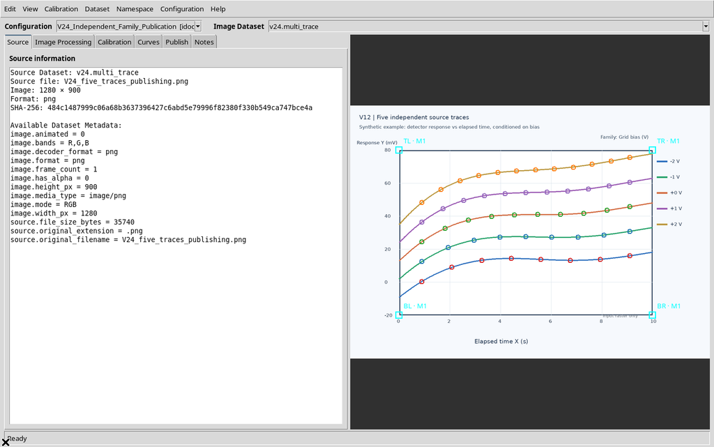
The file measures 1280 × 900 pixels. The presence of five lines in the figure does not automatically produce five numerical curves: association with the source, calibration and acquisition of the points are required.
2. Defining the Common Scientific Calibration
In the Calibration tab, set the quantities Elapsed time and Detector response, with units s and mV respectively. The limits are X = 0–10 s and Y = −20–80 mV.
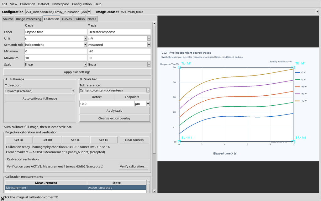
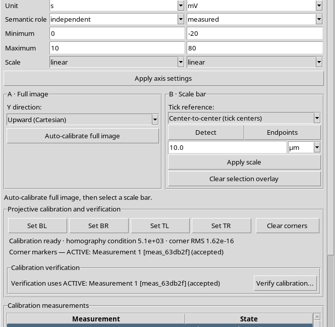
Select the four corners of the original rectangle and accept the measurement. The same transformation is valid for all five curves because they share the same image and the same axes.
3. The Difference Between a Curve and a Dataset
A curve is a series of scientific points with its own identifier. A Dataset is the canonical object published by GX-TXT, which can contain several curves.
In independent mode, five curves can therefore be collected in a single tabular Dataset. The Dataset must keep both the coordinates of the points and a field stating which curve each row belongs to.
4. Creating the First Independent Curve
In the Curves tab, keep This configuration is a numerical curve family disabled. Press New curve and give the first line a name.
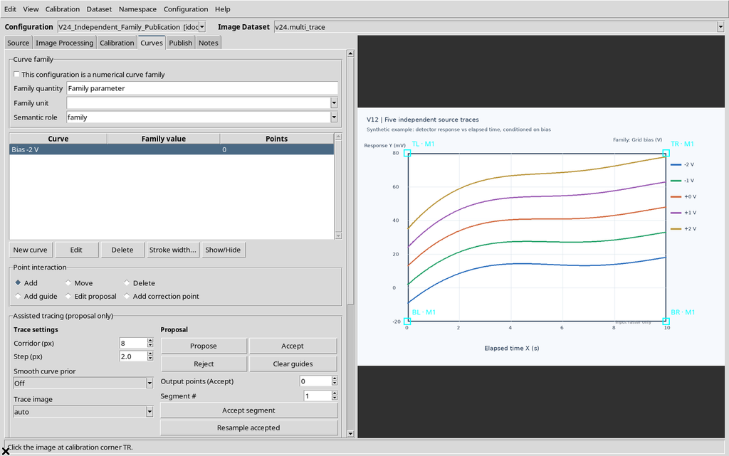
The name is descriptive. The scientific identifier of the curve is assigned internally by the framework and must not be reconstructed from the text of the name.
5. Adding a Second Curve
Repeat New curve for the second trace.
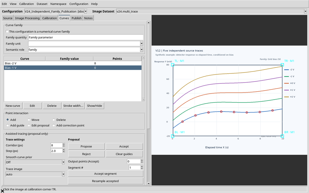
Each new curve appears in a separate row and can be selected to acquire, correct or display only its own points.
6. Adding the Other Three Curves
Create the following curves as well, keeping the relationship with the respective traces in the figure.
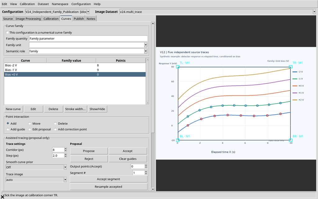
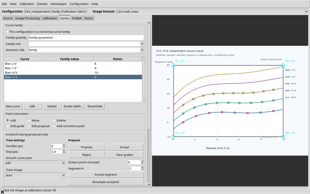
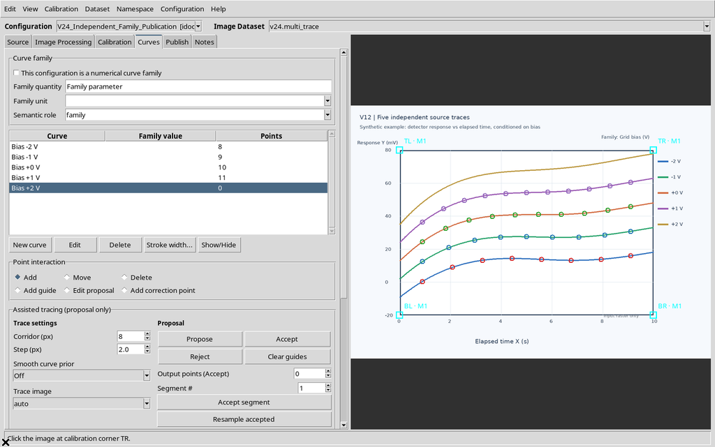
The five names report the conditions shown in the legend, but in this first mode there is not yet a real numerical family_value parameter: the values in the name are only text.
7. Acquiring the Manual Points
Select one curve at a time, use the Add mode and click on the corresponding stroke in the raster.
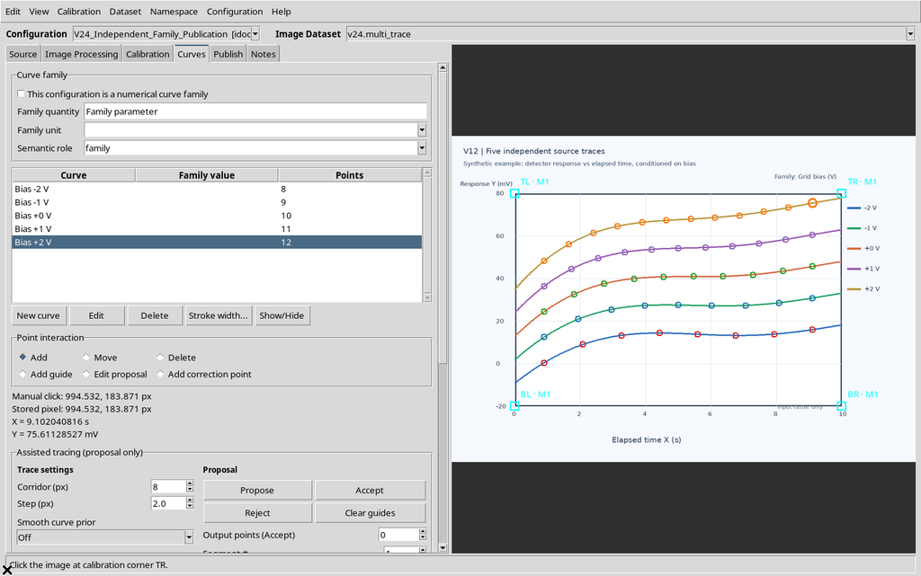
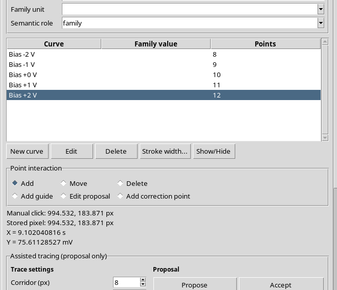
In the example the five traces have 8, 9, 10, 11 and 12 points respectively, for a total of 50 scientific points. The different number of points does not prevent representing them as standalone curves.
8. Identifying and Ordering the Points
The series has its own curve_key. Each point has a point_order, which in this configuration starts from zero within the series.
| Teaching curve | Points | Internal indices |
|---|---|---|
| Bias −2 V | 8 | 0–7 |
| Bias −1 V | 9 | 0–8 |
| Bias 0 V | 10 | 0–9 |
| Bias +1 V | 11 | 0–10 |
| Bias +2 V | 12 | 0–11 |
Do not assume that curve_name is a unique key: it is an editable label. Do not assume either that point_order always matches an ordering by X: the behavior depends on the policy chosen in Digitizing.
9. Preparing the Independent Publication
Open the Publish tab. Select the only accepted calibration and set a Publication base Dataset ID distinct from that of the source.
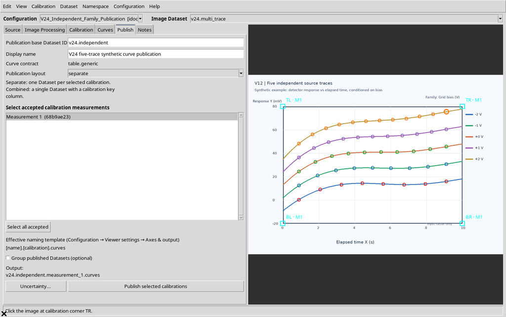
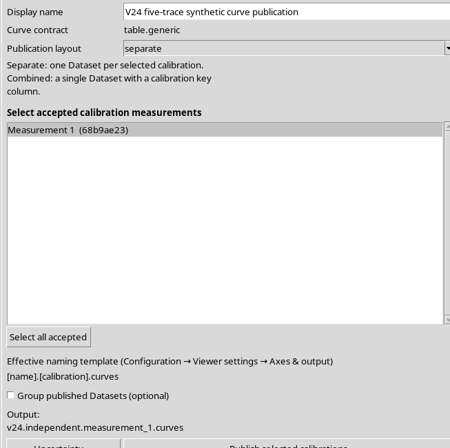
For this workflow we use the separate layout and a single calibration realization. We are not comparing several calibrations or creating a Dataset Group.
10. Publishing the Table.generic Dataset
Press Publish selected calibrations. GX-TXT checks the source, the calibration and the structure of the rows, then registers the canonical output.
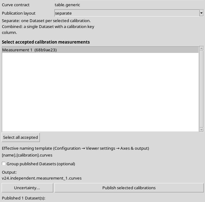
The result contains 50 numerical rows in the table.generic contract, even though there are five curves.
11. Opening the Result from the Dataset Catalog
In the Session Dataset browser the new numerical Dataset is available. Select it and open it with the native command.
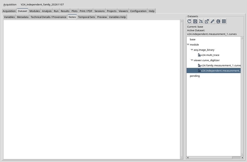
The result stays independent of the Curve Digitalizer Interactive Document. To view the rows there is no need to keep open the window in which they were created.
12. The Plot Tab of the CORE Scientific Viewer
The CORE Scientific Dataset Viewer offers a Plot tab and a canonical table.
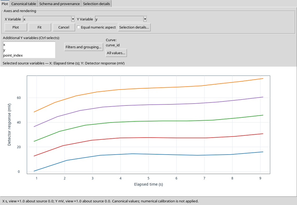
The generic plot does not replace the semantics of the curves: a consumer must recognize curve_key and distinguish the series, instead of indiscriminately connecting all the X/Y points of the table.
13. The Long Format of Independent Data
Open Canonical table.
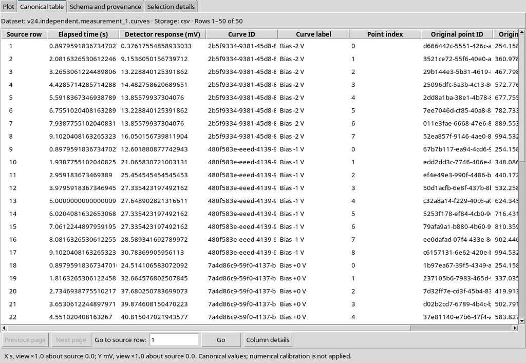
In the implementation examined, the publication includes the technical variables x, y, curve_id, curve_label, point_index, point_id, pixel_x and pixel_y. Each row represents one point.
These technical names are useful for reading the example, but future tools should resolve the columns through the public semantic roles.
14. The Independent Semantic Contract
The publication keeps metadata identifying the independent mode, the table.generic contract, the original image and the calibration.
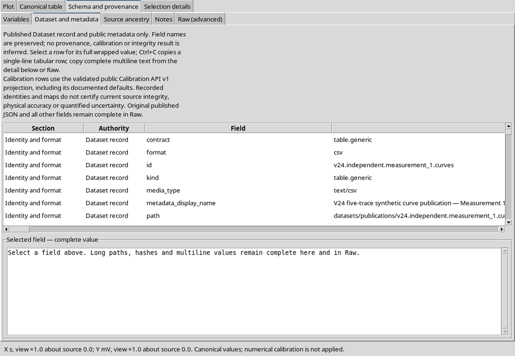
The main roles are:
| Stable role | Meaning |
|---|---|
| x, y | Calibrated scientific coordinates |
| curve_key | Opaque identity of the curve |
| curve_name | Visible label of the curve |
| point_order | Order of the point in the curve |
| raster_x, raster_y | Pixel coordinates of the original image |
The opaque key is the basis of the grouping. The title of the curve can change without necessarily changing its identity.
15. Variable Schema v3 of the Independent Dataset
The CORE Variables section lists eight variables, including the raster coordinates.
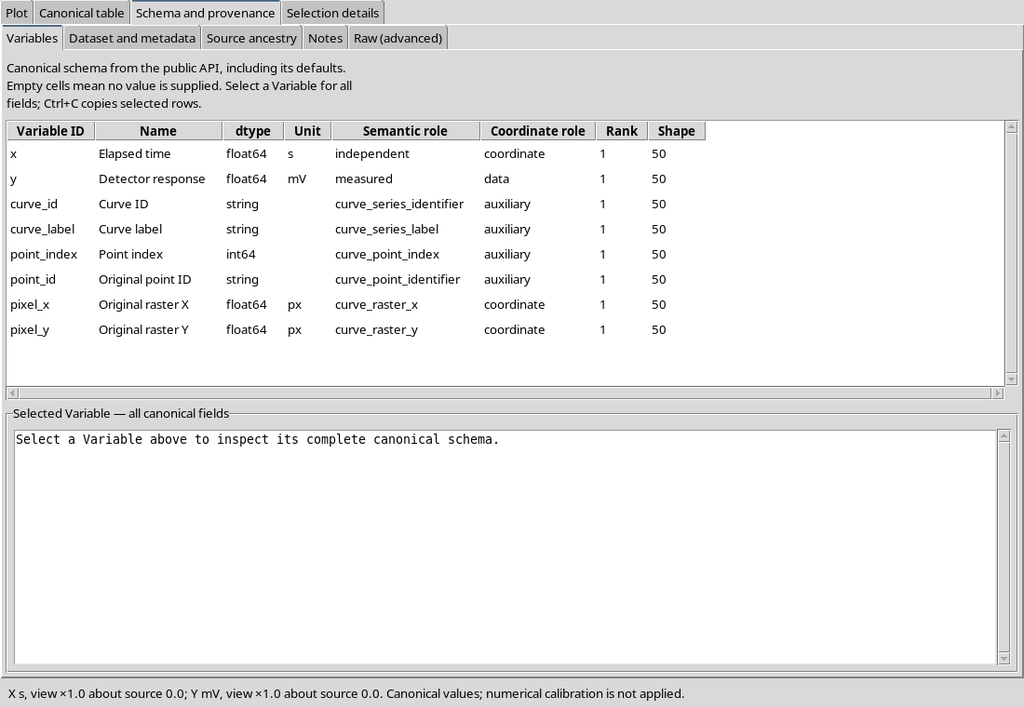
Selecting the curve identifier field you can check its text type.
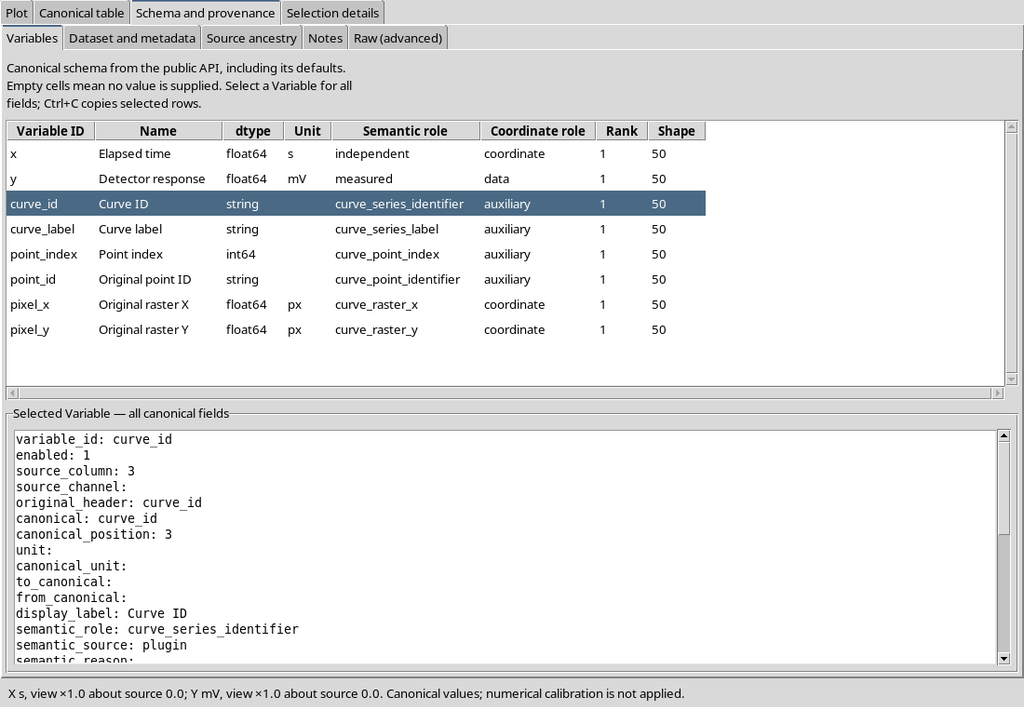
This publication has no numerical family_value column. A label containing “−2 V” is not enough to turn the structure into a family.
16. Enabling Numerical Curve Family
Go back to the Digitalizer Curves tab and enable This configuration is a numerical curve family.
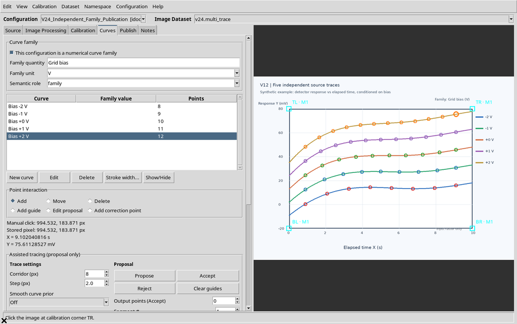
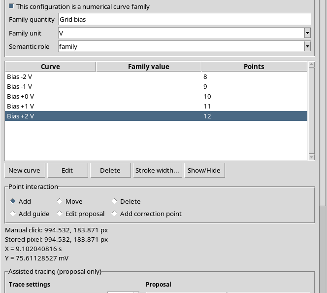
The example uses Grid bias as the quantity name, V as the unit and family as the scientific role. Enabling it changes the type of output intended, but neither deletes nor recreates the fifty points already accepted.
17. A Family Requires Real Numerical Parameters
Trying to publish right away, when the curves have no numerical value, the Viewer shows an error.
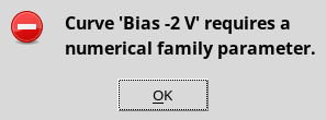
The parameter cannot be inferred from the title “Bias −2 V”. The title is free text: the value must be recorded in the dedicated field, with its unit.
18. Opening Edit Curve to Assign the Parameter
Select the first curve and press Edit.
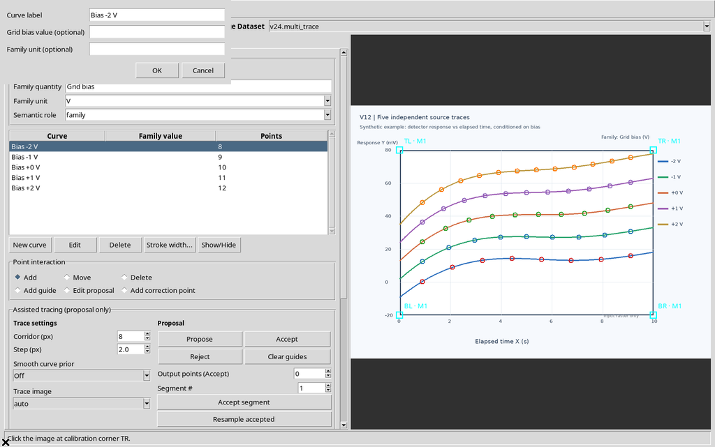
In the dialog, enter the value of the parameter for the curve.
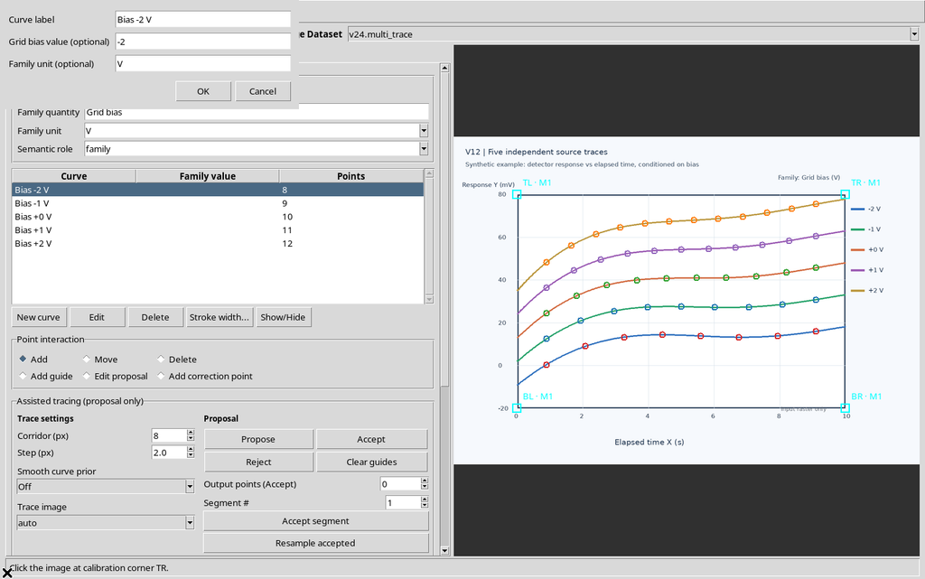
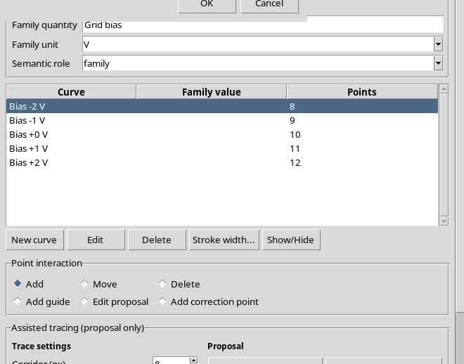
The first condition is −2 V. The parameter belongs to the series and will be repeated in the rows of that series when the family is published.
19. Assigning the Other Values
Repeat the procedure for the remaining traces: −1 V, 0 V, +1 V, +2 V.
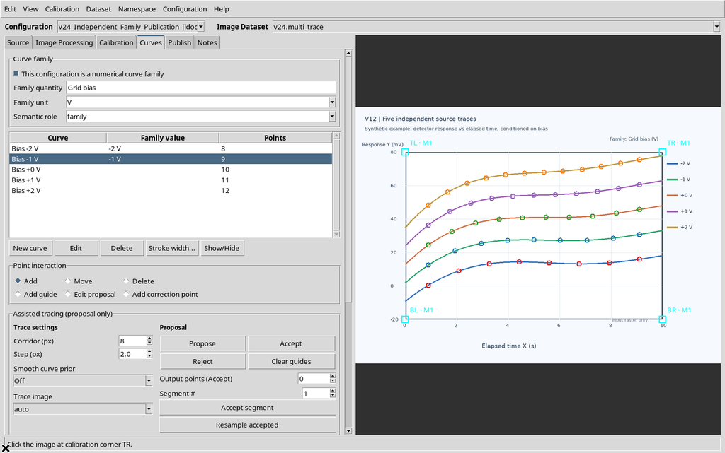
The values are not new measurements of the Y variable: they describe an external condition associated with each curve.
20. Checking the Units of the Curves
In the example, a deliberately wrong test assigns the last curve the value 2 with the unit mA, while the family is defined in V.
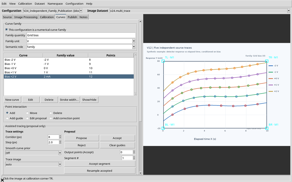
The GUI blocks the publication.
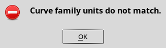
The check prevents conditions expressed in incompatible declared units from being combined in a common numerical column.
21. Correcting the Unit of the Fifth Curve
Open Edit curve again and correct its unit to V.
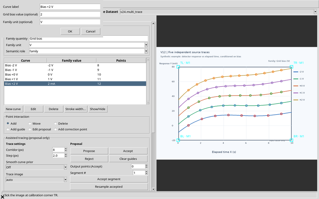
There is no need to move or digitize again the twelve points of the fifth series: the change concerns only the description of the parameter.
22. Checking the Ready Family
The Curves table now shows all five numerical conditions correctly expressed in volts.
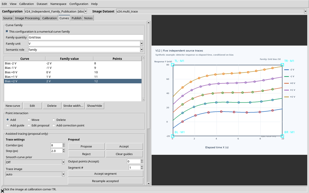
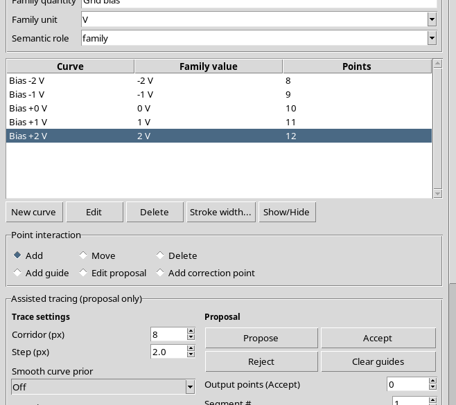
The counts stay 8, 9, 10, 11 and 12. The grouping is still associated with the identities of the five curves.
23. Preparing a Second Output ID
Open Publish, keep the same accepted calibration and choose a new base ID intended for the family Dataset.
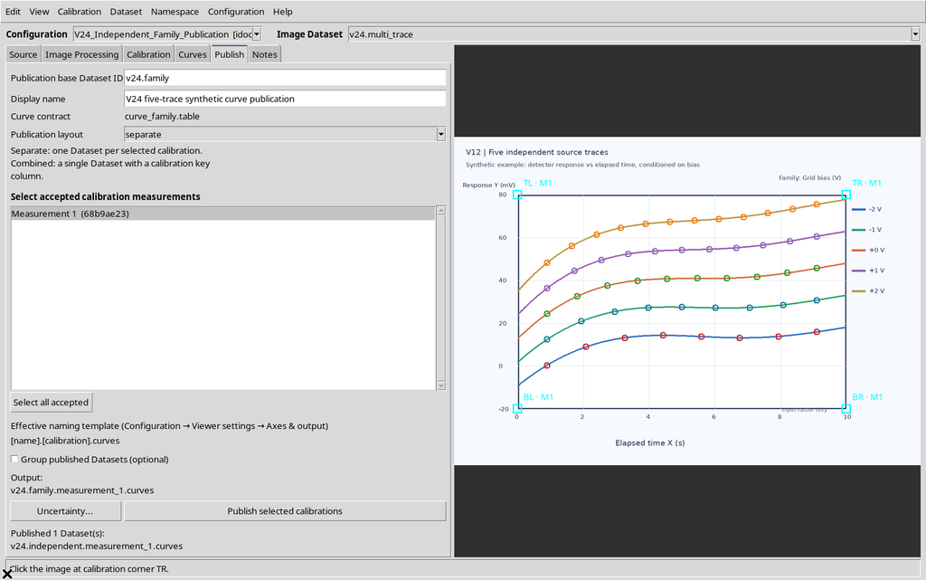
Using a different ID avoids confusing the independent result with the new numerical_family result.
24. Publishing Curve_family.table
Press Publish selected calibrations.
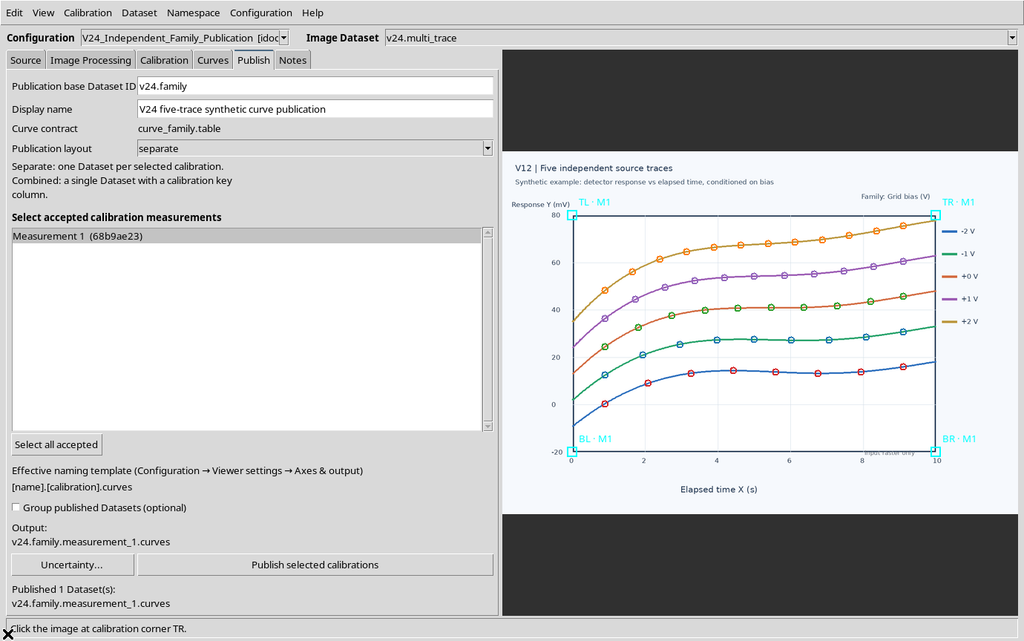
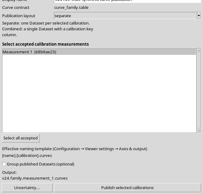
The result now has the curve_family.table contract, with 50 rows and a numerical column for the Grid bias condition. The X/Y scientific samples are those already digitized.
25. Viewing the Family from the Browser
The Dataset browser shows both outputs, identified separately.
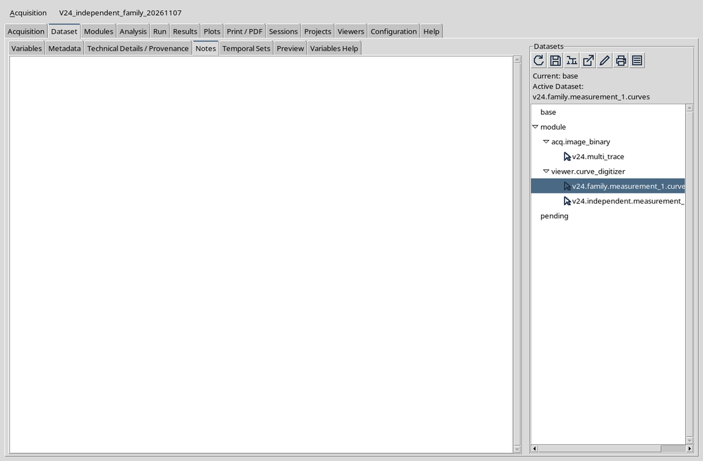
Opening the family Dataset brings up the CORE Scientific Dataset Viewer.
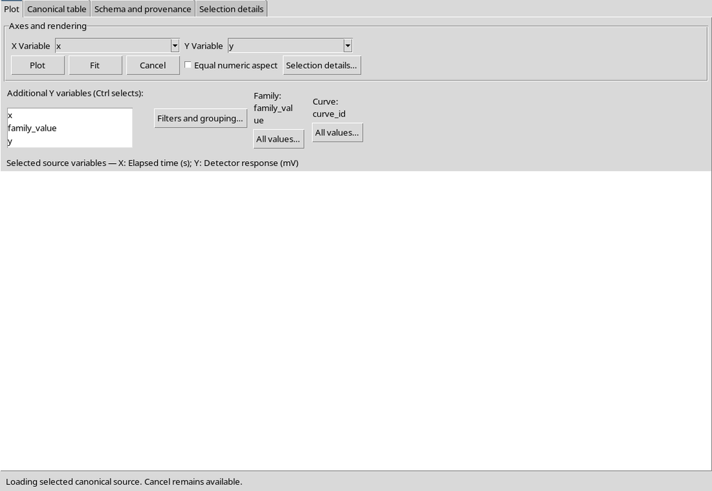
The correct scientific interpretation does not depend on the window name or on the generic plot, but on the curve_family.table contract and on the semantic roles.
26. The Canonical Table of the Family
The canonical table now shows the family_value column.
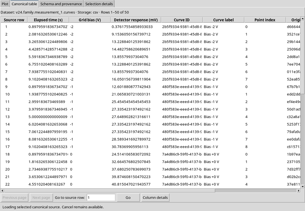
For every point of a given curve the parameter value is repeated: for example, the Bias −2 V curve keeps family_value = -2 in all eight of its rows.
27. A New Column, Not New Points
Comparing the two Datasets row by row shows that the common fields are identical: scientific X/Y, raster coordinates, label, curve identifier, point identifier and order.
| Property | Independent curves | Numerical family |
|---|---|---|
| Contract | table.generic | curve_family.table |
| Mode | independent | numerical_family |
| Rows | 50 | 50 |
| Curves | 5 | 5 |
| Canonical variables | 8 | 9 |
| Numerical parameter | Absent | family_value |
| Grouping key | curve_key | curve_key |
The new column changes the meaning of the rows; it is not a second experimental acquisition.
28. The Structured Provenance of the Dataset
Open Schema and provenance to read the contract of the family result.
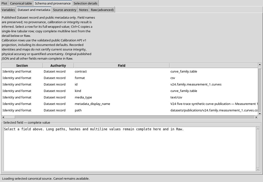
The metadata identify the source image, its SHA-256 fingerprint, the calibration transformation and the roles of the variables. The provenance must be read together with the data, not reconstructed from the colors of the plot.
29. Nine Variables in the Family
The Variables tab shows nine variables, compared with the eight of the independent publication.
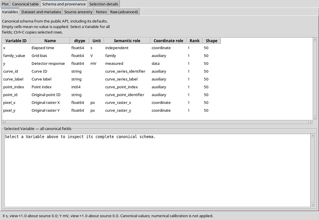
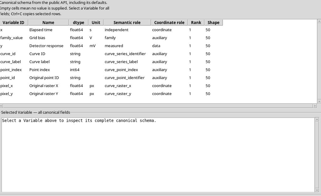
The additional variable is of type float64, has unit V and role family. The X and Y coordinates keep the units s and mV respectively, with no change of axis.
30. Checking the Source Ancestry
The Source ancestry tab lets you check the link between the result and its original data.
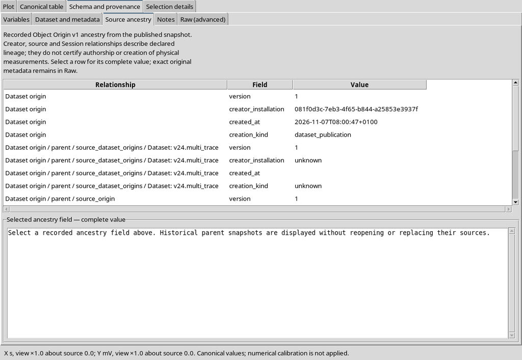
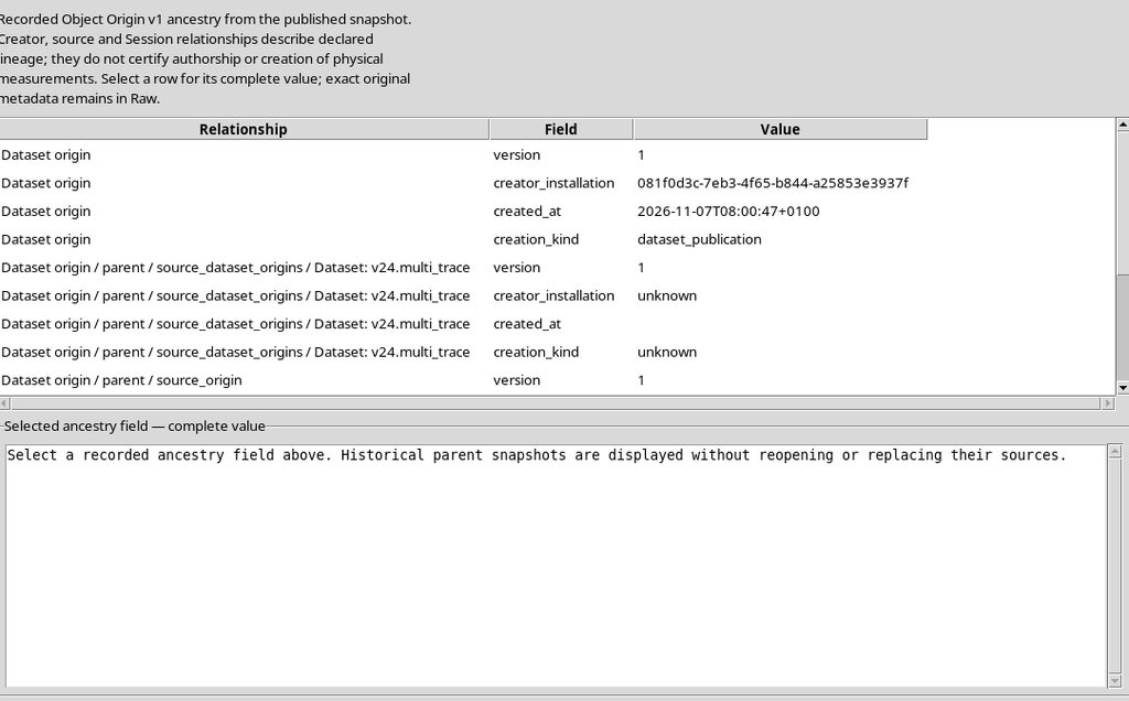
In the example both publications keep the same fingerprint of the original image and the same SHA-256 of the calibration. No two different images were generated and the calibration was not repeated.
31. The Family_parameter Role in the Variable Schema
Selecting the family_value variable in the CORE shows its description.
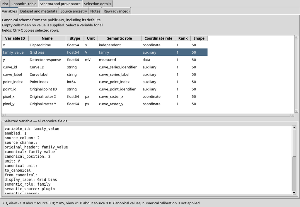
Its stable semantic role is family_parameter. The numerical parameter describes the condition of the series, not the X time and not the measured Y response.
32. Why Curve_key Cannot Be Replaced by the Parameter
The family Dataset still contains a text variable identifying the curve.
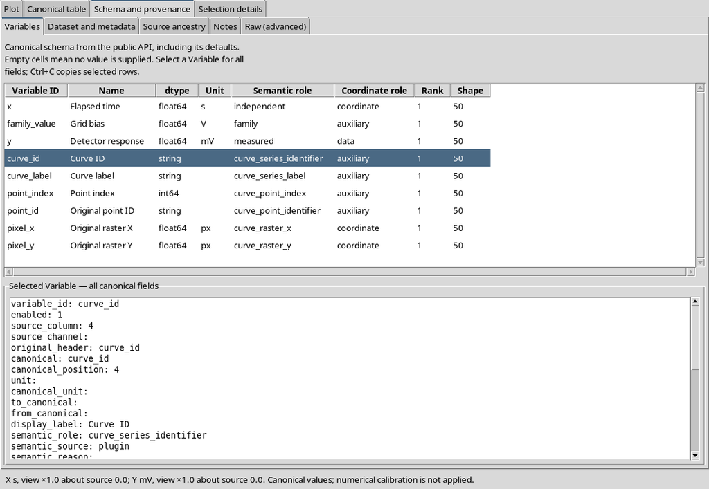
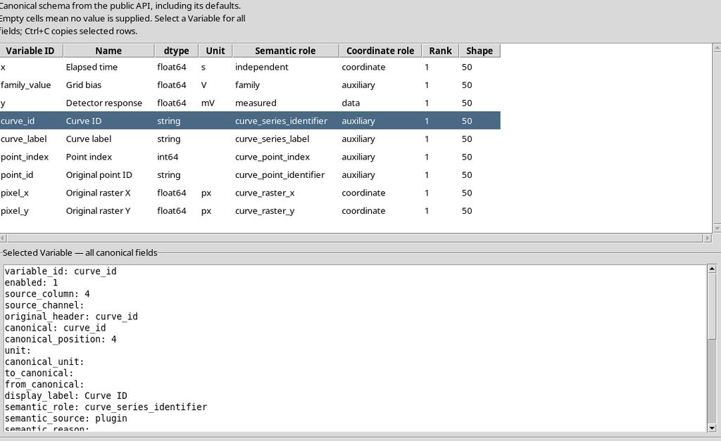
curve_key serves to separate the series. family_parameter describes a numerical condition and is not a primary key: in other experiments two curves might share the same parameter value and still be two different curves.
33. The Point Order Is Internal to the Curve
The point_order field is a zero-based integer.
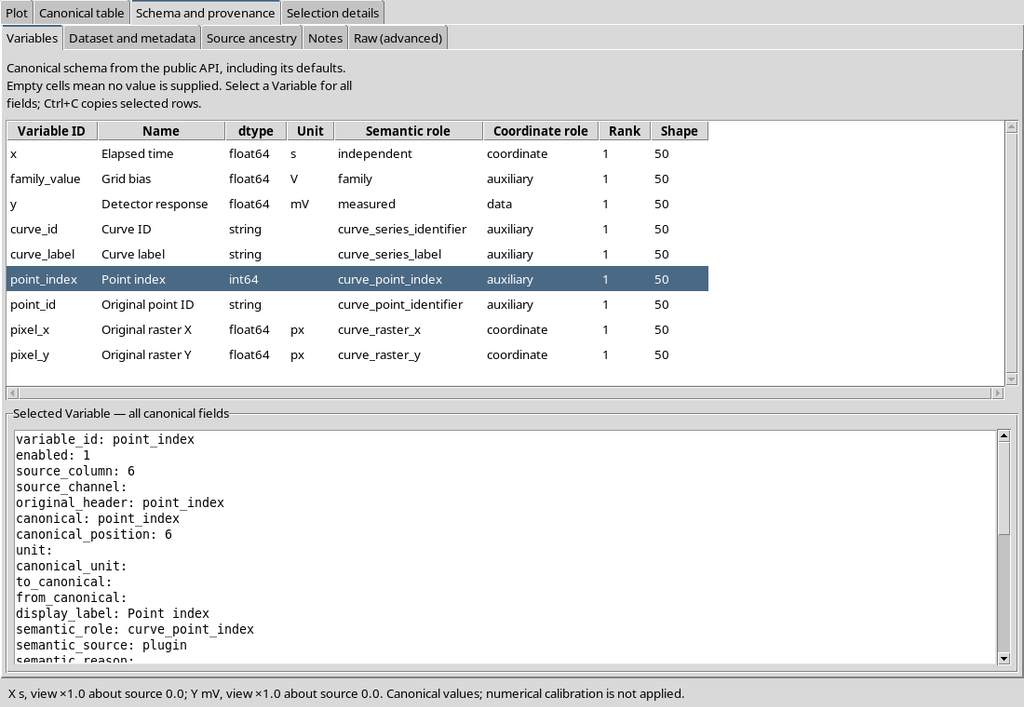
In the example the sequences are 0–7, 0–8, 0–9, 0–10 and 0–11, each within its own curve. Sorting the records globally by X or by the parameter is not equivalent to rebuilding the sequence defined by the operator.
34. The Raster Coordinates Remain Available
Both published Datasets keep the coordinates of the original pixels, in addition to the calibrated X/Y.
These references are essential for scientific checking: they make it possible to compare a numerical point with the original trace without having to approximately reconstruct the geometry from the displayed plot.
The source used is a synthetic image; the agreement of the clicks with its mathematical formulas does not measure the accuracy of an instrument.
35. Temporarily Going Back to Independent
The This configuration is a numerical curve family control can be disabled in the current configuration.
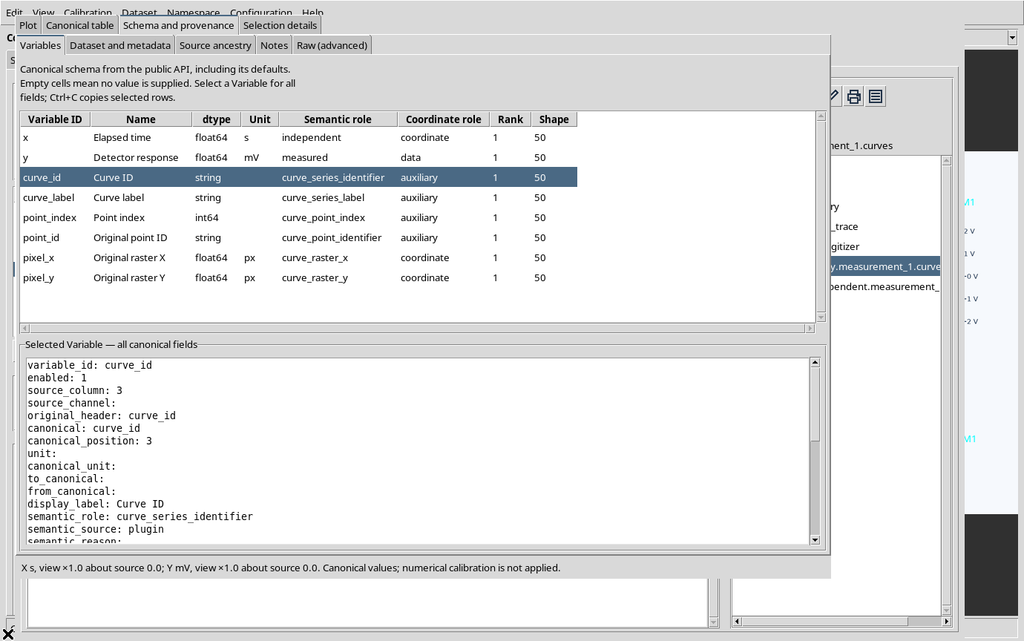
The five traces and their points stay available. Datasets already published are not deleted or reinterpreted by a change of mode in the still-editable document.
36. Re-enabling the Family
Re-enabling the checkbox, the five numerical conditions are found again.
In the example the sequence of points, the identifiers and the coordinates stayed unchanged, both in the document and in the outputs already consolidated.
37. Saving, Closing and Reopening
Use Configuration → Save configuration, close the Viewer normally and reopen it from the same Session.
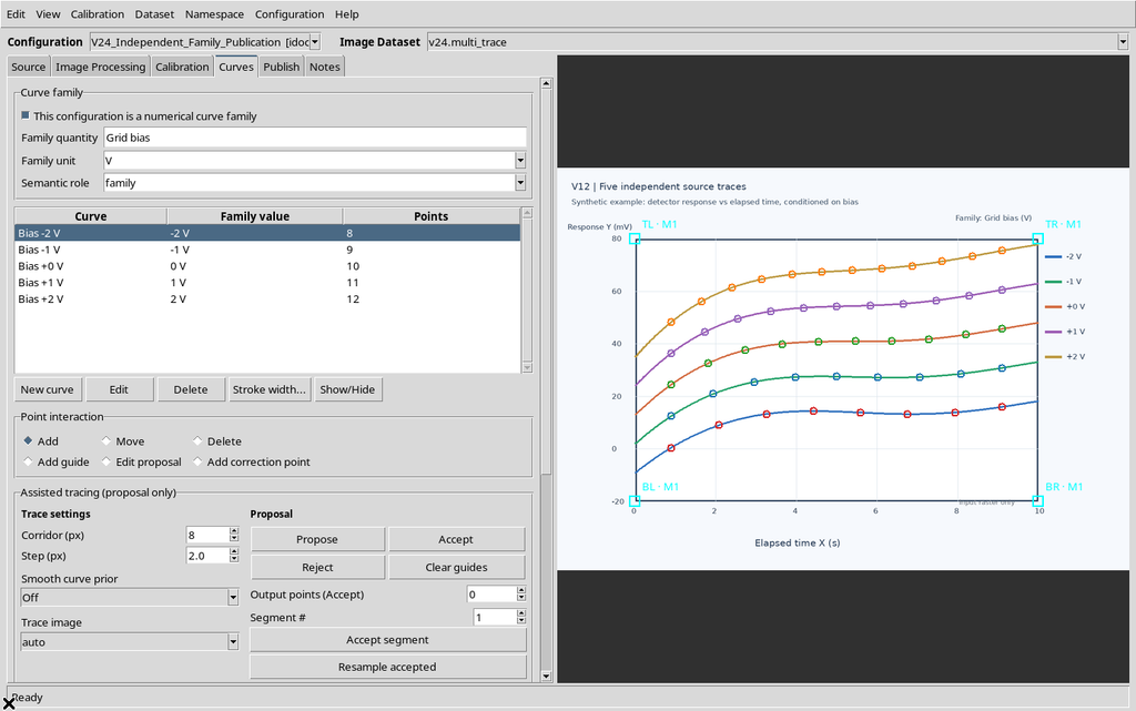
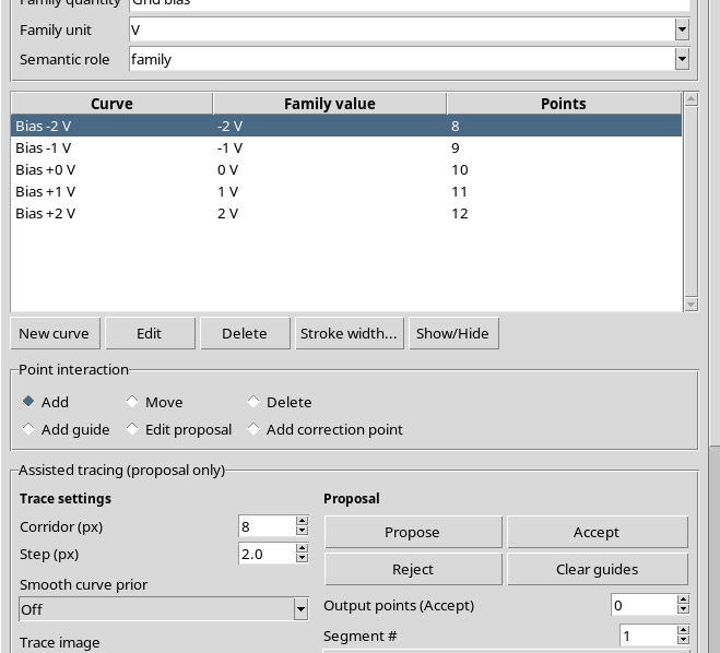
The five curves, the values −2, −1, 0, +1 and +2 V and the fifty original points come back.
38. Persistence of the Outputs and the Source
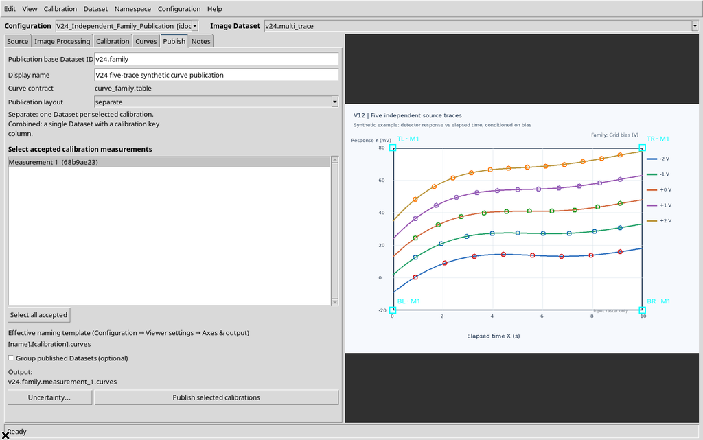
The Publish tab shows the family publication plan, still associated with the accepted calibration.
The Source tab confirms that the source Dataset is still the original one.
The public APIs keep reading the two Datasets already published, with unchanged identity and SHA-256. This persistence is distinct from the save operation of the current configuration.
39. Reading the Columns Through the Public APIs
Programs that consume the result should not infer scientific roles from technical names such as curve_id, curve_label or family_value, because they might evolve. The versioned Curve Digitalizer API resolves the associations from the metadata and from Variable Schema v3.
A Tcl example in the GX-TXT environment, with the appropriate Session open:
# Activate the public Curve Digitalizer Dataset Schema API.
::GX::modulePublicApiActivate viewer.curve_digitizer CURVE_DIGITIZER_DATASET_SCHEMA_API_v1

set dataset_id "example.family.curves"
set manifest [::GX::CurveDigitizerDataset::read $dataset_id]

# Resolve semantic roles rather than assuming CSV header positions.
set curve_key_variable [dict get $manifest columns curve_key]
set point_order_variable [dict get $manifest columns point_order]
set x_variable [dict get $manifest columns x]
set y_variable [dict get $manifest columns y]

# A numerical family also declares a repeated numeric parameter.
if {[dict get $manifest mode] eq "numerical_family"} {
    set parameter_variable [dict get $manifest columns family_parameter]
}

# Read the original raster positions through the bounded public API.
set batch [::GX::CurveDigitizerDataset::rasterPoints $dataset_id "" 0 100]

# Group rows by curve_key, then order within each group by point_order.
The rasterPoints function returns the source coordinates in a bounded read. The roles returned by the API are linked to the canonical variables actually published.
40. Independent Curves and Families Are Not Synonyms
The independent mode is appropriate when the curves must be considered distinct series, with no declared common numerical parameter.
The numerical_family mode is appropriate when the variation of a quantity, such as Grid bias in volts, has an explicit scientific meaning for each series.
Do not convert to a family just because the curve names contain numbers: consistent units and a real parameter are required. Conversely, do not consider two Datasets as new independent measurements if they come from the very same acquisition of points.
41. Recommended Operating Procedure
- Import the original raster and accept the scientific calibration.
- Create a curve for each trace, assigning clear names and acquiring the points in the correct series.
- Check the counts and the grouping by curve, without using the name as an identifier.
- For independent curves, keep the family disabled and publish the table.generic Dataset.
- For a family, enable This configuration is a numerical curve family and enter the quantity, the unit and the numerical value of each curve.
- Correct missing values or incompatible units before publishing.
- Publish the curve_family.table Dataset with a distinct identity.
- Open the two results in the CORE and compare the canonical rows and the Variable Schema.
- Use CURVE_DIGITIZER_DATASET_SCHEMA_API_v1 to resolve the columns, curve_key for grouping and point_order for the sequence.
- Save, close and reopen; check the source, the number of points, the family parameter and the persistence of the Datasets.
Conclusion: converting from independent curves to a numerical family changes the semantics of the published table, not the pixels or the original coordinates. Correctly distinguishing curve identity, point order and family parameter lets later analysis tools use the data without confusing traces or experimental conditions.