

Snapping, Scientific Ordering and Undo/Redo History
This guide explains how to use Snap to dark, Radius, Monotonicity, Point ordering source, Undo and Redo. The procedures are carried out on a synthetic raster with dark reference points and two numerical curves, to show how pixels, scientific coordinates and point order are kept.
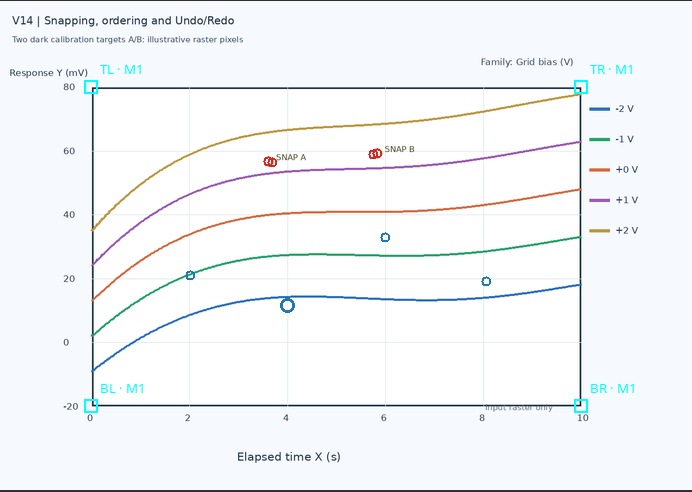
1. A Synthetic Raster with Two Dark References
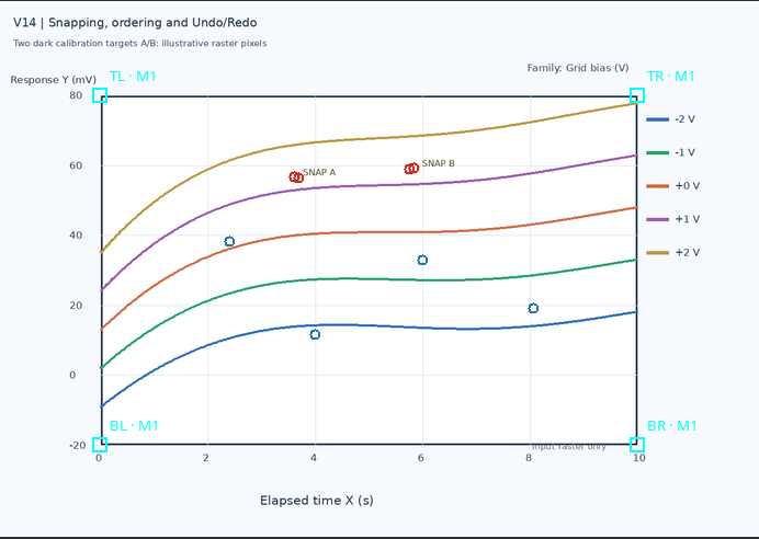
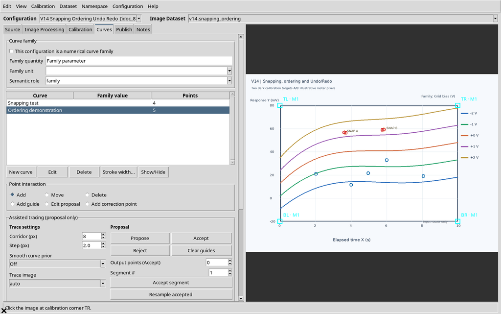
The source is a synthetic scientific PNG of 1280 × 900 pixels, with five colored traces and two small black reference points named SNAP A and SNAP B.
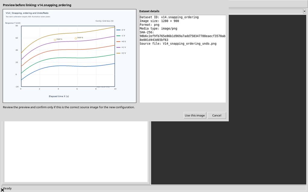
The references were added to the test raster solely to distinguish the click made by the operator from the point stored after snapping. They are not published numerical curves and do not represent instrument data or calibration standards.
2. Scientific Calibration Before Pixel Selection
The image was imported as a single canonical image.raster Dataset, in an example Session. Curve Digitalizer used an accepted four-point calibration, with axes Elapsed time X = 0–10 s and Detector response Y = −20–80 mV, both linear.
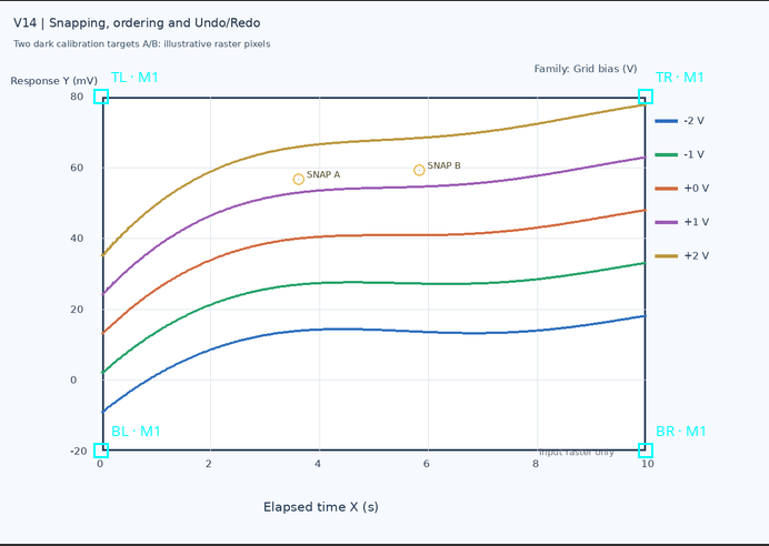
Provisional points, test points and ordered points are always transformed using the same four corners. This prevents coordinate differences from being attributed to an uncontrolled change of scale or raster.
3. Where the Controls Are
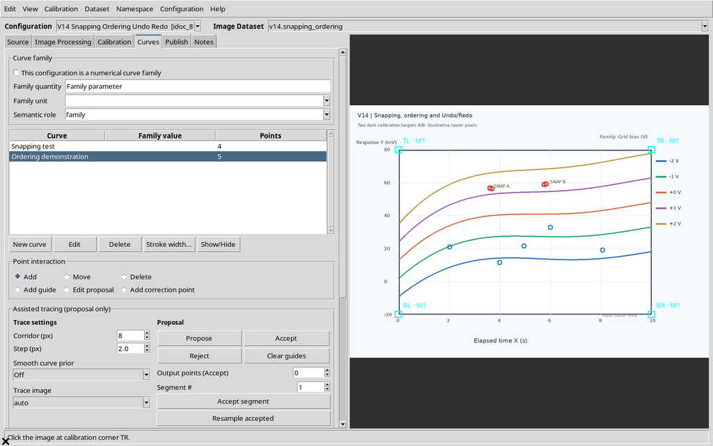
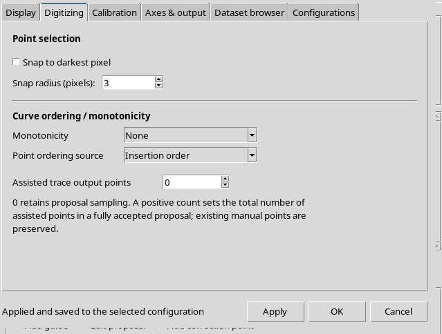
The Curves tab contains Display and snapping, with the Snap to dark checkbox and the Radius spinbox. The same parameters are also available from Configuration → Viewer settings… → Digitizing, where the labels become Snap to darkest pixel and Snap radius (pixels).
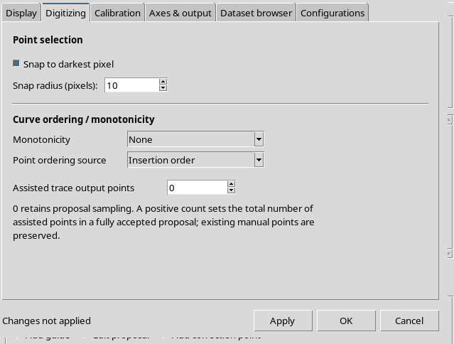
The same Digitizing tab offers Monotonicity and Point ordering source. The window keeps a draft of the settings separate from the actual Apply button.
4. Manual click Is Not Always the Same as Stored pixel
The Viewer keeps two distinct pieces of information: the source pixel where the actual click landed, i.e. Manual click, and the pixel chosen by the snapping criterion, i.e. Stored pixel. The latter is transformed into the scientific X/Y coordinates.
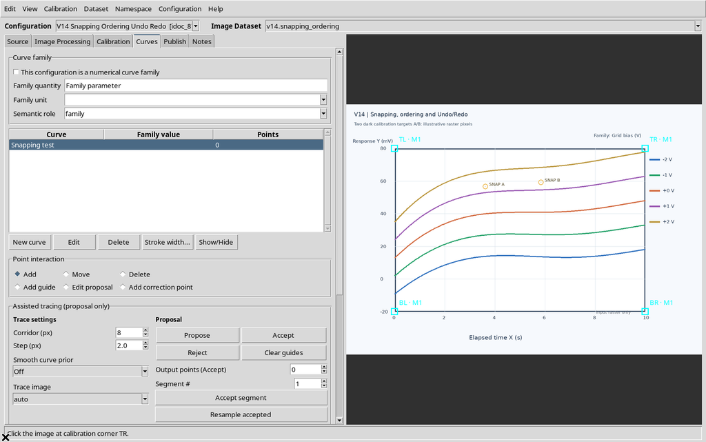
Snapping does not change the original pixels of the PNG, does not rewrite the four corners and does not automatically give a physical meaning to a dark region.
5. Snapping Disabled, Even with Radius 10
The snapping checkbox was disabled while Radius = 10. A click made near SNAP A kept exactly the manual pixel.

The Workspace recorded Manual click = Stored pixel = (506.475; 296.216) px. The radius is a stored preference, but it stays inactive until the Snap to dark control is enabled.
6. Snapping Enabled with Radius Zero
Snap to dark was then enabled, but with Radius = 0. A click near SNAP B still stayed at the manual point.
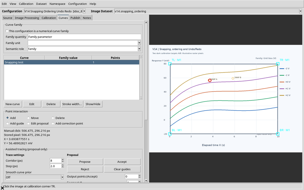

The stored value turned out to be (692.489; 281.482) px, identical to the click. Enabling the checkbox without a positive radius does not cause any shift.
7. Snapping with Radius 10: Reference A
With Snap to dark enabled and Radius = 10, the same click near SNAP A found the original black pixel at the center of the reference.
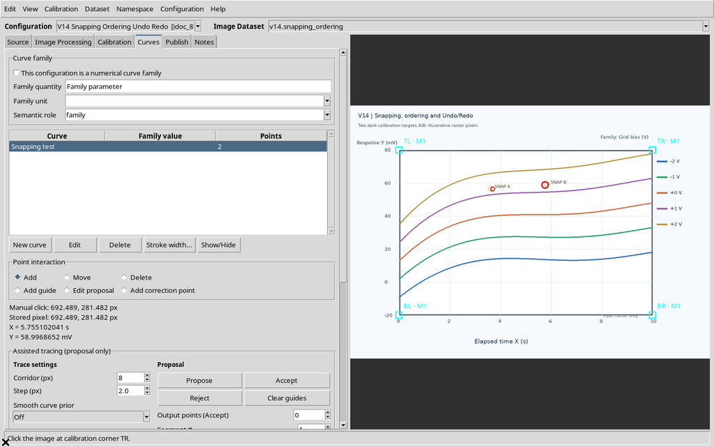
The GUI showed:

| Field | Value |
|---|---|
| Manual click | (506.475; 296.216) px |
| Stored pixel | (500; 295) px |
| Shift in the raster | about 6.588 px |
| Resulting scientific X | about 3.622 s |
| Resulting scientific Y | about 56.696 mV |
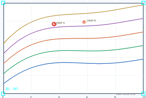
The point keeps its scientific identity and two different source coordinates. The original raster is not modified: only the scientific pixel associated with the added point changes.
8. Snapping with Radius 10: Reference B
The command was repeated on the second reference. The manual click near B had coordinates of about (692.489; 281.482) px; the stored point became (700; 280) px.

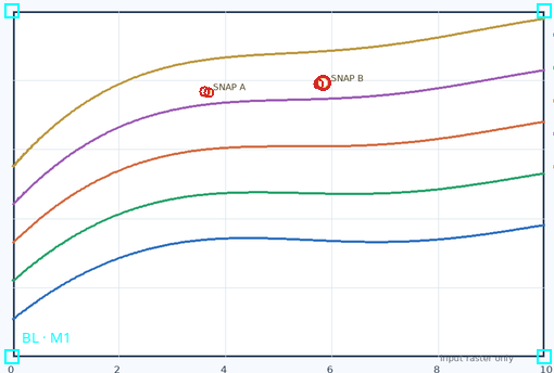
The shift is about 7.656 source pixels. The new scientific coordinates are about X = 5.838 s and Y = 59.249 mV.
9. Independent Check of the Darkest Pixel
To check the result without relying only on the Viewer label, the PNG was independently converted to grayscale intensity. All pixels within the set radius around the click were analyzed, reproducing the search window of the installed model.
For both references, the search rectangle contained a single pixel with minimum intensity 0: (500,295) and (700,280) respectively. These were exactly the pixels chosen by the Viewer.
This is not a test of intelligent curve recognition: it demonstrates a local search for the intensity minimum, with the candidate closest to the click chosen when several pixels are equally dark.
10. The Radius Is Expressed in Source Pixels
The program analyzes the image in grayscale and computes the search rectangle around the pixel of the original image. A radius of 10 px therefore corresponds to source pixels, not to ten pixels of a resized screenshot or to ten physical units.
The Viewer zoom changes the mapping of the mouse to the raster, but does not replace the scientific calibration. Snapping can pull the click towards text, a grid or a competing trace: it is a local aid, not a curve recognizer and not a measure of uncertainty.
11. Four Test Points, Four Documented Conditions
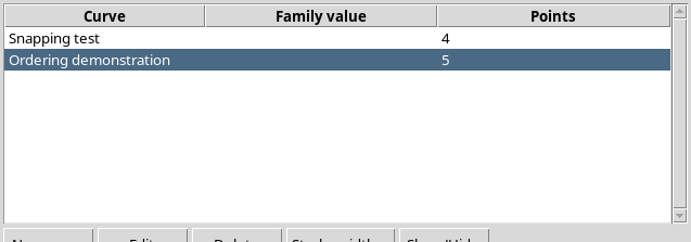
The first curve, Snapping test, contains four points: two inserted without position correction and two acquired with snapping to the darkest pixel enabled.
The IDs of the four records are distinct. The manual and stored coordinates coincide only in the cases without effective snapping. No numerical scientific table was published; the points live in the Digitizer Configuration.
12. Edit → Undo: Undoing the Last Insertion
The Edit menu contains Undo (Ctrl+Z) and Redo (Ctrl+Y). After the fourth point was created, the actual Edit → Undo command was run.
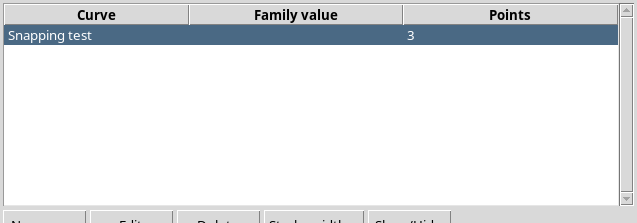
The curve count went from four to three, removing the last record from the scientific configuration. No other point changed.
13. Edit → Redo: Restoring the Same Point
With Edit → Redo the last point reappeared. No new search for dark pixels was run.
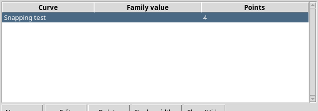
The Workspace keeps the same UUID, the same manual_click_pixel, the same pixel and the same X/Y values that were present before Undo.
14. Keyboard Shortcuts and Focus
To undo and redo changes you can also use the Ctrl+Z and Ctrl+Y shortcuts, provided the Viewer has the focus.
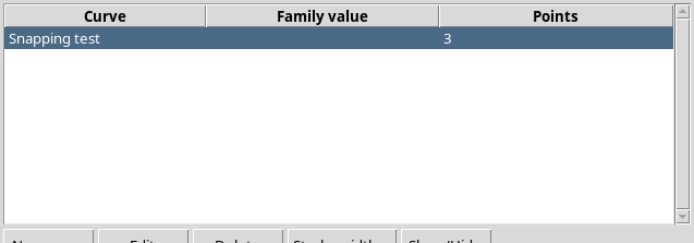
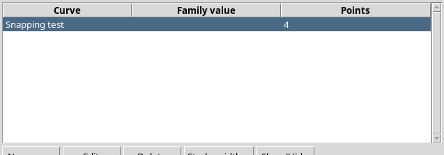
The sequence goes from four to three points and back to four, restoring the same record. Ctrl+Z and Ctrl+Y require the focus to be in the correct window.
15. A Second Curve to Demonstrate Insertion Order
A second object, Ordering demonstration, independent of Snapping test, was created with snapping left disabled.
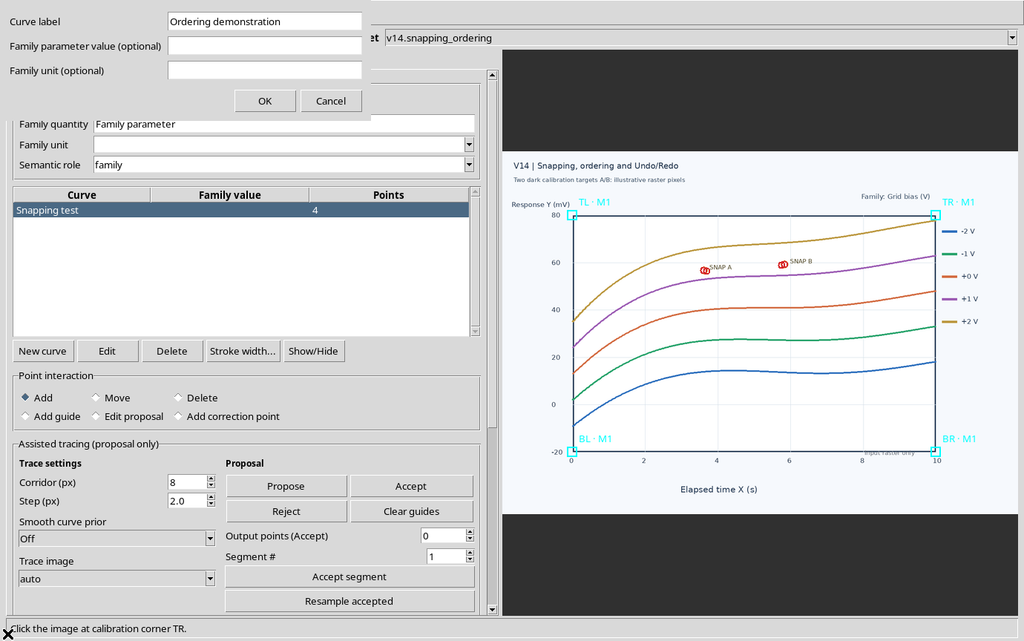
In the default mode, Monotonicity = None and Point ordering source = Insertion order, four points were inserted with deliberately unordered nominal X coordinates: 8, 2, 6, 4 s.
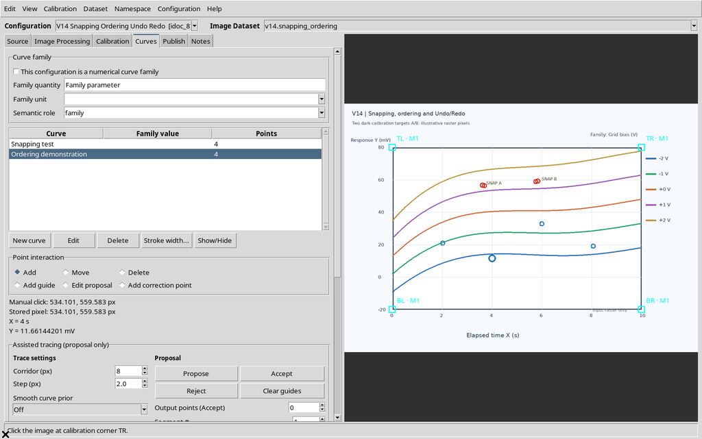
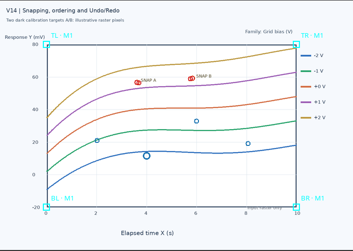
The framework kept exactly this insertion sequence, without automatically reordering the points by X or Y.
16. Why the Point Sequence Matters
In a curve that folds back, a closed path, a time scan or a parametric graph, the sequence of the points can have a meaning independent of their X position. Sorting automatically by X without being asked would alter that sequence.
In GX-TXT the operator can keep Insertion order or explicitly choose Sort by X or Sort by Y. The control concerns the scientific list of points, not a new detection of pixels.
17. Sort by X: First the Draft, Then Apply
Configuration → Viewer settings… → Digitizing was opened and the Sort by X option selected. Before Apply was pressed, the Workspace still kept the previous policy.
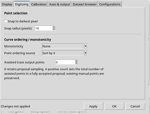
Only after Apply did the status Applied and saved to the selected configuration appear, and the persistent policy became source = x.
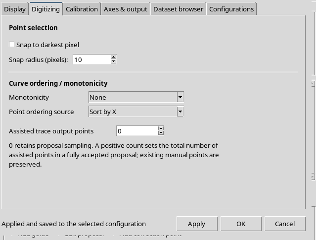
This difference between the values shown in the dialog and the settings actually saved is important: it is not enough to select an entry in the combobox and close the window without applying it.
18. Sort by X Keeps the Data but Changes the Positions in the List
After it was applied, the four points of the second curve were sorted by increasing scientific X: approximately 2, 4, 6, 8 s.
The UUIDs, the source pixels, the manual origin and the calibrated values of the four records were exactly the same: what changed is the position of the records in the sequence. The two curves of the configuration are each sorted according to their own scientific coordinate.
19. Monotonic in X Forces Sort by X
Selecting Monotonic in X, the Point ordering source entry was set automatically to Sort by X, already while the draft was being edited.
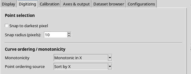
The software thus prevents a contradictory combination of an axis declared monotonic and an incompatible ordering source. No new data were generated and the position of the points was not changed.
20. Changing the Ordering Can Cancel the Monotonicity
While X monotonicity was selected, Sort by Y was chosen in the second combobox. The GUI automatically set Monotonicity = None.
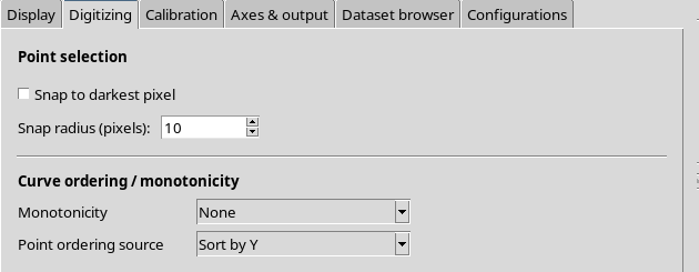
This is intentional Viewer behavior: a declared X monotonicity cannot stay active together with an ordering by Y. Clearing the incompatible declaration is neither an error nor a change of pixels.
21. Monotonic in Y Forces Sort by Y
Selecting Monotonic in Y, the Viewer automatically set Sort by Y.
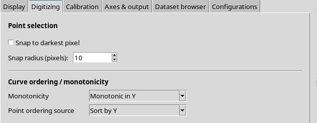
After Apply, the Workspace confirmed monotonicity = y and source = y. This control expresses an ordering and constraint policy for the tools that use it; on its own it does not prove that the source function is mathematically monotonic.
22. Y Ordering Without X Monotonicity
The four points of the second curve had increasing Y after the reordering, but their scientific X values were about 4, 8, 2, 6 s.
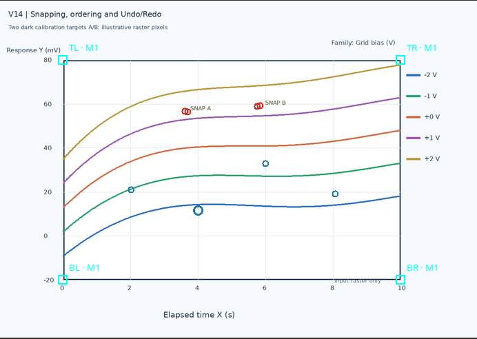
This is an observable difference between sorting by the Y quantity and sorting by X. The interface must not present the new sequence as if it came from new clicks or from moved markers.
23. Undo and Redo of the Ordering Change
With Edit → Undo the previous Sort by X policy was restored, with the same records in increasing X sequence. With Edit → Redo, Monotonic in Y and the increasing Y sequence came back.
The operation includes the configuration model and the order of the points, not just the text of the combobox. All scientific identifiers and coordinates stayed identical.
24. Move Reorders the Point According to the Active Policy
While Monotonic in Y was active, one of the points of Ordering demonstration was dragged to a position with a higher Y.
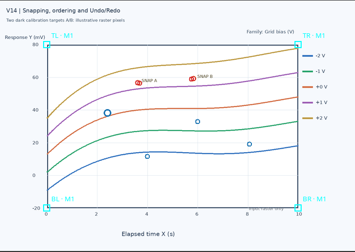
The point kept its UUID, but its X/Y coordinates were recalculated and its record moved to the last position because it now had the highest Y. The source raster and the other three points of the curve were not modified.
25. Undo/Redo of a Move Also Restores the Order
Undo restored the previous position and order.
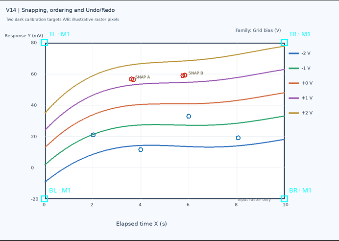
Redo applied the move and the related reordering again.
26. After Undo, a New Edit Discards the Old Redo Branch
The move of a point was undone and a new point was immediately added to the curve with Add.
The subsequent Redo attempt no longer restored the old Move: the new insertion had broken off the previous branch of the history.
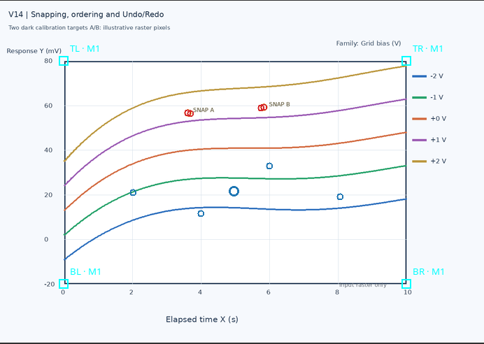
Undo and Redo of the new point, on the other hand, stayed available and kept the new UUID.
In practical terms, the history is a sequence of reversible states; a new change after Undo creates a different continuation, it does not keep two competing branches.
27. The Valid Snap radius Range Is 0–25
In the Digitizing tab, Snap radius = 26 was entered and Apply pressed. The GUI showed the error:
Snap radius must be between 0 and 25 pixels.
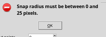
The Workspace is not modified by an invalid value. The radius can be set back to 3 px and snapping disabled through the settings.
28. Going Back to Insertion order Does Not Rebuild the Past
After the list had been sorted by Y, the operator set Monotonicity = None and Point ordering source = Insertion order again, saving with Apply.
The future policy went back to insertion, but the points were not restored to the original click sequence 8–2–6–4. The list still held the order resulting from the sort already applied.
This is consistent with the implementation: in insertion mode the software does not run a new sort, but it does not keep a second, permanent history of the old indices. To recover the previous order you need an appropriate Undo, as long as the history of the same run is available.
29. Save, Close, Reopen: Persistent Data, Temporary History
The configuration was saved with Configuration → Save configuration, closed normally and reopened from the Viewers → Digitalizer catalog in the same Session.
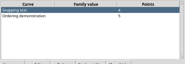
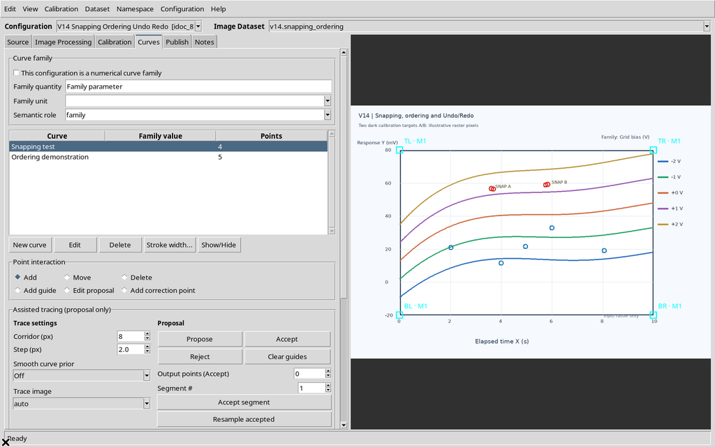
What was recovered: the original source Dataset, one accepted four-corner calibration, two curves with four and five points respectively, all the UUIDs and the manual/stored pixels, the X/Y coordinates, Snap to dark disabled, Radius 3 and the None / Insertion order policy.
Trying Undo and Redo in the new run of the Viewer, no change was made.
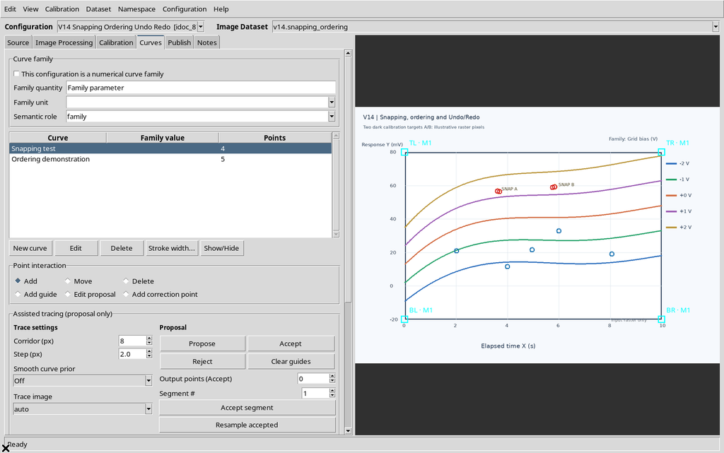
The Undo/Redo history is not saved as part of the Datasets or of the canonical Workspace: it is transient and belongs to the current process. It must not be confused with the normal persistence of the scientific points.
30. Operating Procedure
To use these functions: select a curve, calibrate the raster and set Snap to dark and Radius according to the resolution of the image. In the Digitizing panel, choose Monotonicity and Point ordering source according to the scientific nature of the curve, press Apply and read the confirmation. Use Undo/Redo before closing the Viewer to recover reversible changes; save the configuration to keep its data, not to keep the history stack.