

Step, Monotonicity and Guide Order
Assisted tracing in the GX-TXT Curve Digitalizer makes it possible to follow a visible line in a scientific image. Two choices affect the result: the sampling step Step (px) and the criterion by which the guides are traversed. This guide shows the two controls on a known synthetic curve, so that the visible result can be compared with a reference trajectory.
1. What Step (px) Means
Step (px) controls the nominal distance between the samples the algorithm evaluates along the path indicated by the guides. The unit is the pixel of the original source image, independent of the Canvas zoom and of the physical units defined by the calibration.
In the version described, the field accepts values from 0.5 to 20 pixels, with a default of 2.0. A smaller step offers more candidate points and a denser search; a larger step offers fewer and can skip narrow details. It must not be confused with Smoothness, with the stroke width or with the number of final numerical points chosen for acceptance.
2. Preparing the Image, Calibration and Series
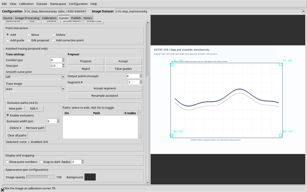
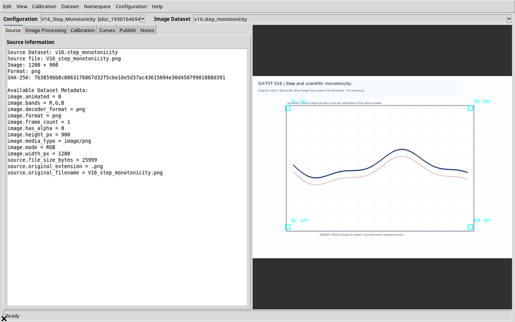
To compare different Steps you need the same Image Dataset, the same calibration and the same target series. The example uses a synthetic raster image of 1280 × 900 pixels with a wavy blue line and a second, light pink stroke shifted with respect to the first. The axis system is X from 0 to 10 s and Y from −20 to 80 mV.
In the Curves tab the series is initially empty: the results of the assistant are still provisional and add no scientific points until the operator uses an acceptance command.
3. Finding the Tracing Controls
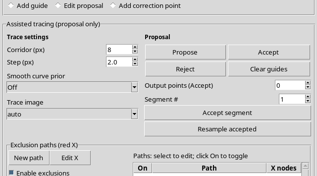
Open Curves, select the series and scroll down to Point interaction and Assisted tracing. Choose Add guide to place the constraints on the raster. The Search corridor (px) and Step (px) fields act on the search; the Propose button generates a new candidate, while Reject deletes the current proposal without clearing the guides.
4. Placing the Guides on the Raster
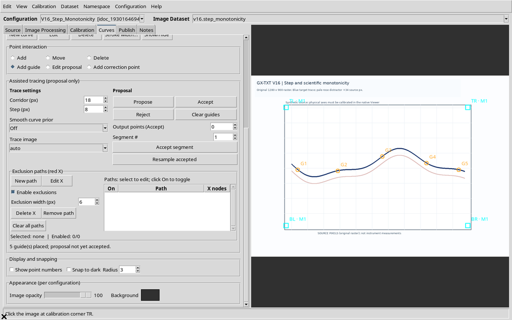
In the example, five clicks along the blue line create G1–G5 in orange. The guides define four consecutive intervals. With None / Insertion order the order of the intervals is the order of the clicks; with a scientific ordering active, the selected axis is followed.
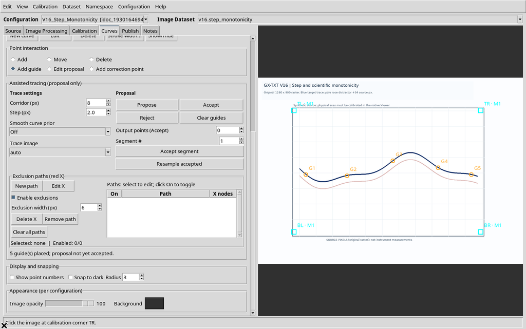
The guides are not points acquired into the series. It is useful to add one where the slope changes, at tight bends and at crossings with unrelated graphic elements.
5. Keeping the Comparison Conditions Fixed
To isolate the effect of Step, all the following tests keep five identical guides, Corridor = 18 px, Smoothness = Off, Trace image = auto selection with no processed preview and the same starting image. Only Step changes: 2, 20, 0.5 and 8 px.
After each change, press Propose again and check the final message. Changing the number written in Step does not, by itself, recompute the previously generated line.
6. Proposal with Step = 2 px
With the default step of 2 px, the panel returns 411 provisional points spread over four segments. The candidate line is drawn over the original image, distinct from the five orange references and from the underlying blue curve.
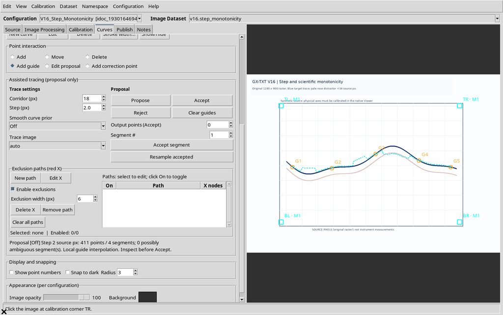
The message states the Step actually used. It is this value, not simply the one now in the field, that must be associated with a proposal already visible.
7. Proposal with Step = 20 px
Setting Step to 20 px and running a new Propose, you get 44 points, still over four segments.
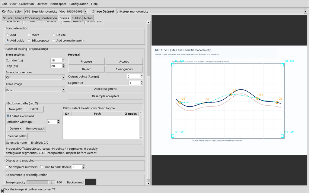
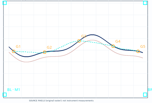
The path is sampled much more coarsely. This is the upper limit allowed by the GUI, not a setting to recommend for every source: fast local shapes, narrow peaks and changes of direction may require a smaller step.
8. Proposal with Step = 0.5 px
At the lower limit of 0.5 px, a new Propose generates 1,636 points over four segments.
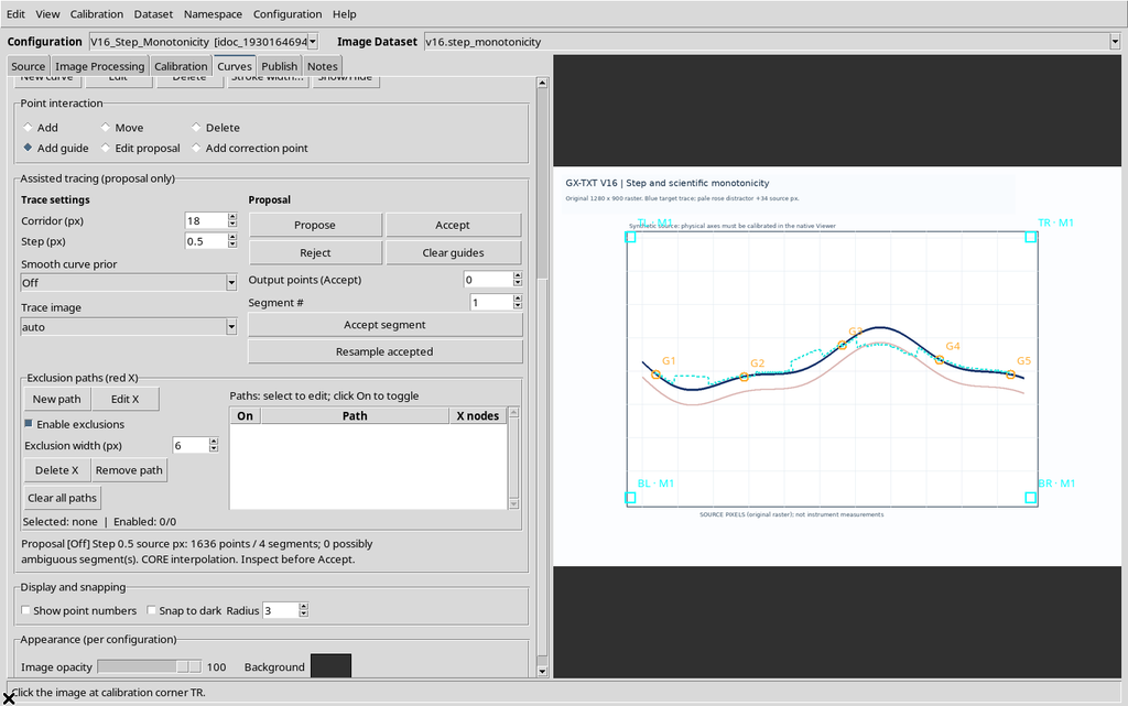
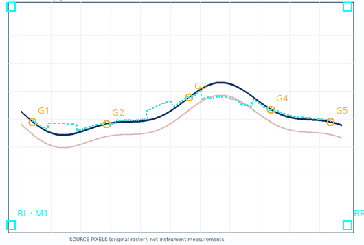
The high number only describes the density of the candidate. It is not equivalent to 1,636 independent measurements and does not certify the accuracy of the curve.
9. An Intermediate Value: Step = 8 px
With Step 8 px the result contains 105 provisional points in four segments.
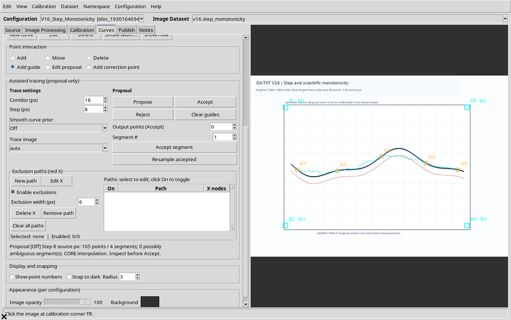
Comparing with fixed parameters makes it possible to decide which level of sampling adequately represents the geometry actually present, without confusing the difference in density with a change in calibration.
10. Number of Points and Fidelity to the Reference
The synthetic blue curve follows a known function in the coordinates of the original image:
y_px(x) = 440 + 58 sin[2π(x−200)/720] + 20 sin[2π(x−200)/305]
The vertical difference between the coordinates of the proposal, read from the Canvas and mapped back to the original pixels, and the known function gives:
| Step | Candidate vertices | Mean absolute deviation | Geometric RMSE |
|---|---|---|---|
| 0.5 px | 1,636 | 14.40 px | 19.63 px |
| 2 px | 411 | 13.78 px | 18.85 px |
| 8 px | 105 | 12.81 px | 17.54 px |
| 20 px | 44 | 16.17 px | 21.74 px |
In this single example Step 8 produces the lowest mean deviation, while Step 0.5 generates many more vertices without reducing the deviation. The errors are geometric distances from a synthetic reference: they are not metrological uncertainties, confidence probabilities or validations on experimental measurements. In general, the proposed path must always be inspected.
11. Step Values Out of Range
Entering 0.49 and pressing Propose, the Viewer shows the message Step must be 0.5..20 original-image pixels. No new proposal is computed with that value.
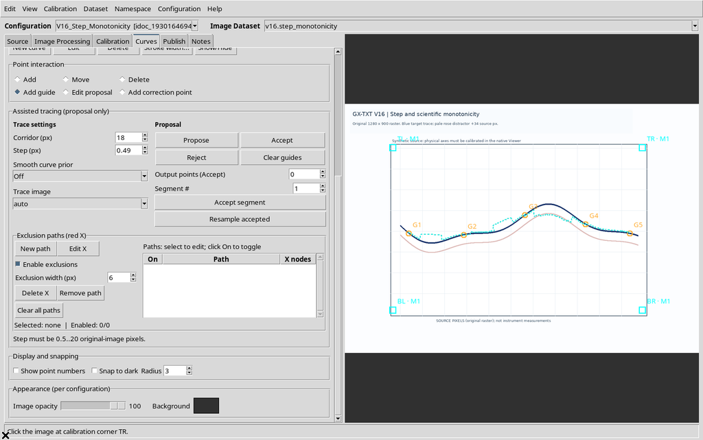
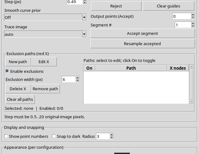
The same happens when entering 21, above the upper limit.

The limit is expressed in original pixels and does not change with the window size or the zoom.
12. Telling the Updated Field Apart from the Proposal Already Visible
If Step is changed after a valid generation, the previous candidate can stay on the Canvas. Even after an out-of-range value is rejected, the line can represent the last correctly completed proposal. To attribute a path to a given parameter, read the summary Proposal […] Step N source px and repeat Propose after every valid change.
The Step error signals that the new request was rejected. A line that stays visible must not be treated as if it had been computed with the new, wrong value.
13. Rejecting the Candidate Without Losing the Guides
Use Reject to delete the current proposal without removing the five orange references.
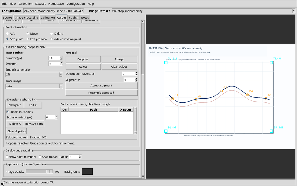
Clear guides is a different command: it deletes the provisional constraints and the proposal. Neither command is equivalent to deleting a series of scientific points already acquired.
14. Two Distinct Concepts: Monotonicity and Ordering
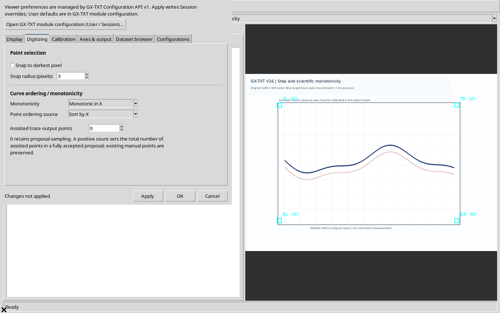
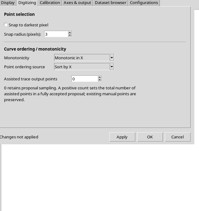
Opening Configuration → Viewer settings → Digitizing you find two distinct fields: Monotonicity and Point ordering source.
| Monotonicity | Point ordering source | Meaning |
|---|---|---|
| None | Insertion order | Free path; click order |
| None | Sort by X | Scientific ordering by X without declaring monotonicity |
| None | Sort by Y | Scientific ordering by Y without declaring monotonicity |
| Monotonic in X | Sort by X | Guide and point policy along X |
| Monotonic in Y | Sort by Y | Guide and point policy along Y |
A simple ordering by X does not prove that the Y quantity is monotonic, and a curve with reversals of direction requires particular care before a monotonic policy is imposed.
15. Guides in Free Insertion Order
With None / Insertion order, five references are inserted in a deliberately non-increasing order along X: first a guide on the right, then one on the left, then other alternating positions. G1, G2 and the following ones follow the clicks and are not reordered automatically.
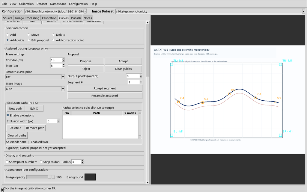
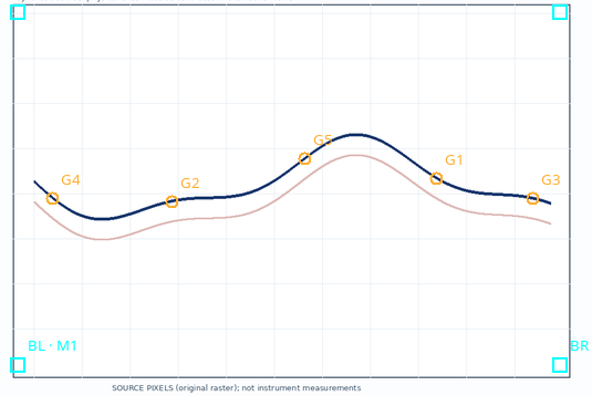
This mode is suitable for contours, paths that go back on themselves and other geometries that cannot be described with a single increasing ordering. Responsibility for the sequence of the intervals stays with the operator.
16. Free Proposal with the Same Guides
With Step 8 px, Corridor 18 px and the five positions inserted in free order, the GUI returns 287 points over four segments.
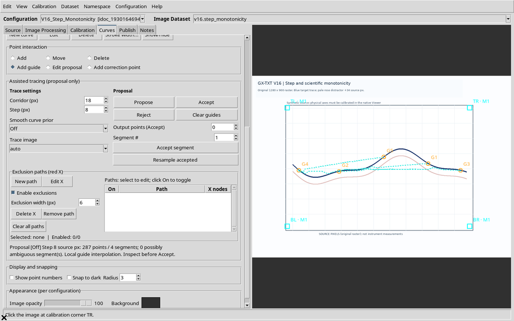
The result differs from the one with X monotonicity even though exactly the same guide points are used. The difference comes from the traversal order, not from a shift of the physical reference.
17. Opening Viewer settings and the Digitizing Tab
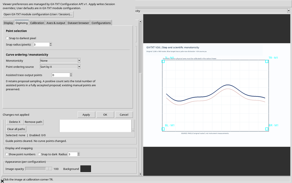
Open Configuration → Viewer settings… and select Digitizing. The initial configuration shows Monotonicity = None and Point ordering source = Insertion order.
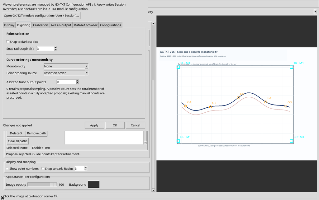
The changes stay in the dialog until Apply is pressed. Read the confirmation message before closing the settings.
18. Enabling Monotonic in X
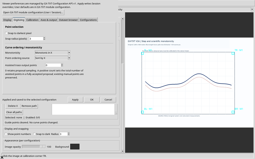
Selecting Monotonic in X, the Viewer automatically sets Sort by X.
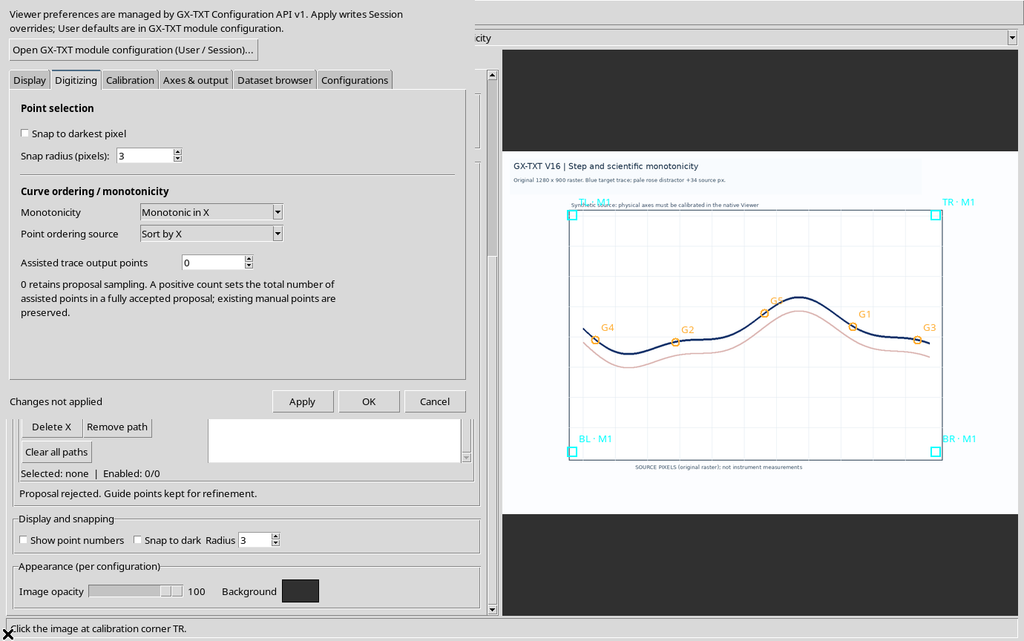
Press Apply to save the policy in the current configuration. The ordering refers to the calibrated scientific coordinate, not simply to the horizontal column of the screen when the image transformation is not trivial.
19. The Same Guides Ordered by X
After enabling the policy, we add the five guides again in the same non-increasing click order used before. This time the labels G1–G5 are assigned in increasing X order.
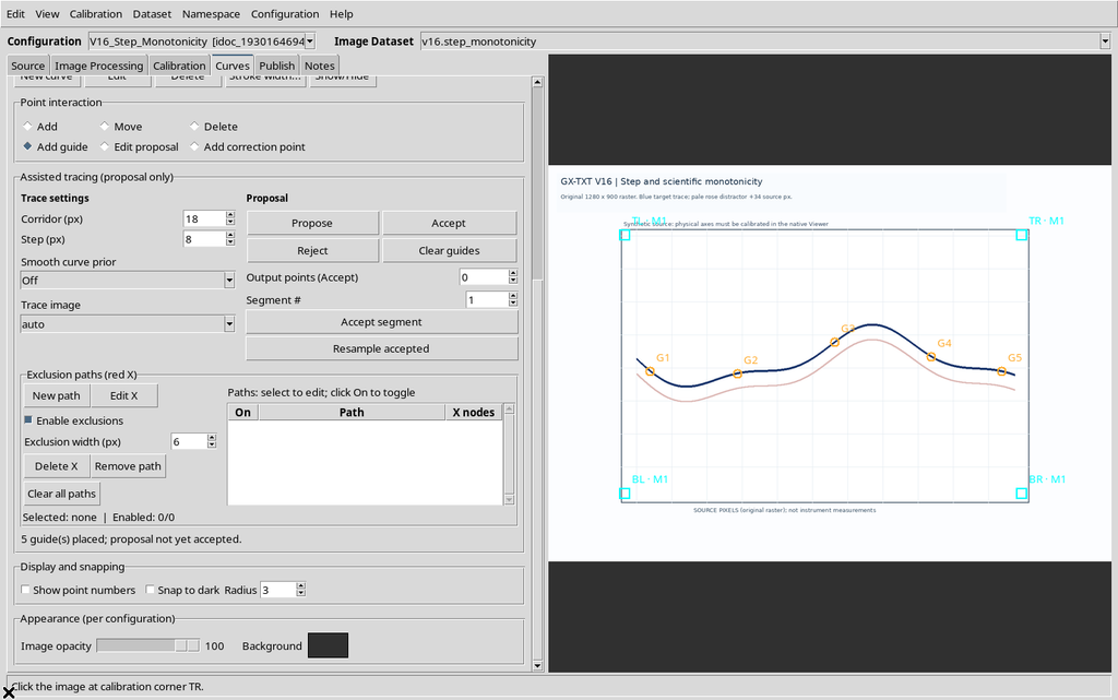
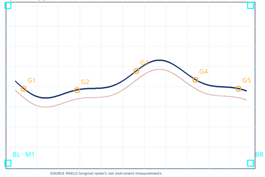
The new Propose with Step 8 returns 105 points over four segments.
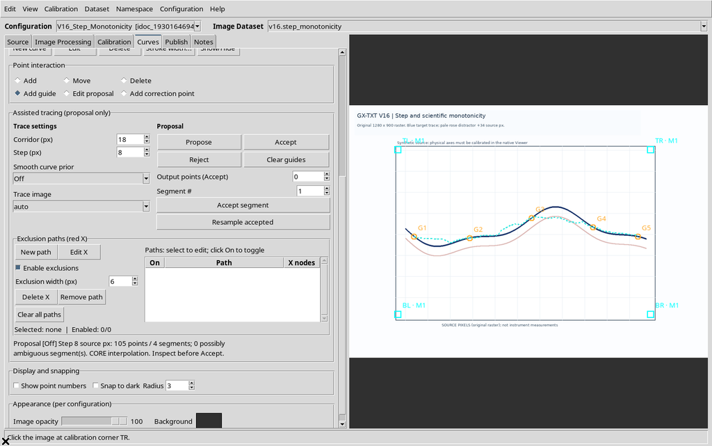
The X policy is appropriate when the curve must be traversed from smaller to larger X. It is not a universal criterion for closed contours or trajectories that turn back horizontally.
20. Enabling Monotonic in Y
Selecting Monotonic in Y, the ordering field switches to Sort by Y.
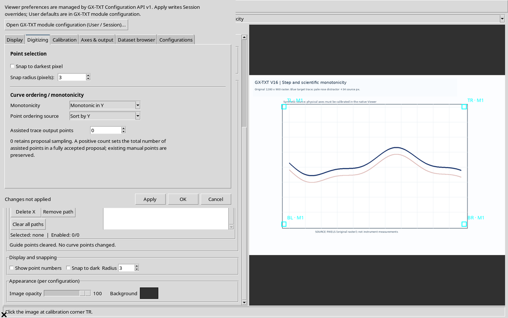
Repeating the previous five clicks, the sequence of the guides changes: G1–G5 now follow increasing scientific ordinate, not the abscissa or the click order.
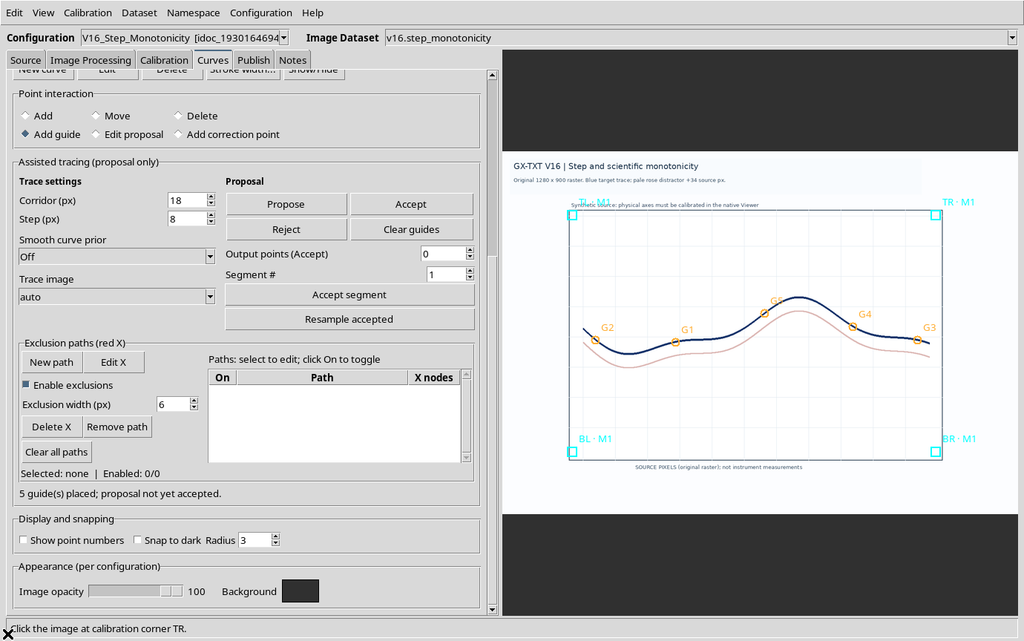
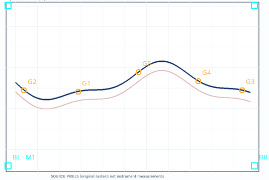
With this configuration the proposal contains 175 vertices over four segments.
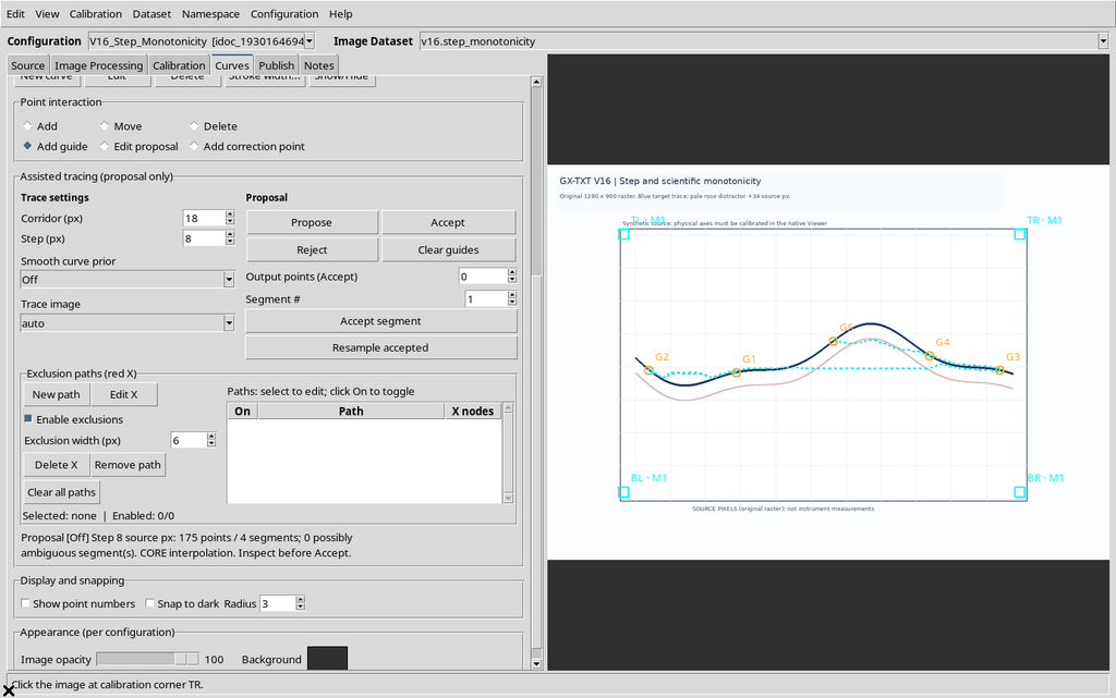
The blue curve used here oscillates in Y: so the monotonic Y constraint does not faithfully represent its overall structure. It is a useful example to understand that the setting must be chosen according to the real geometry of the data, not to get a desired number of points.
21. Ordering by X Without Declaring Monotonicity
While Monotonic in Y is selected, changing Point ordering source to Sort by X sets Monotonicity back to None.
After Apply, when the guides are added in scattered order, they are still arranged by X.
The relationship is therefore asymmetric: declaring a monotonicity imposes the consistent ordering; manually changing the ordering to another axis can remove the monotonic declaration.
22. Back to Free Mode
To work on contours or unordered geometries again, set Monotonicity = None and Point ordering source = Insertion order, then press Apply. This way the operator again determines the sequence through the clicks.
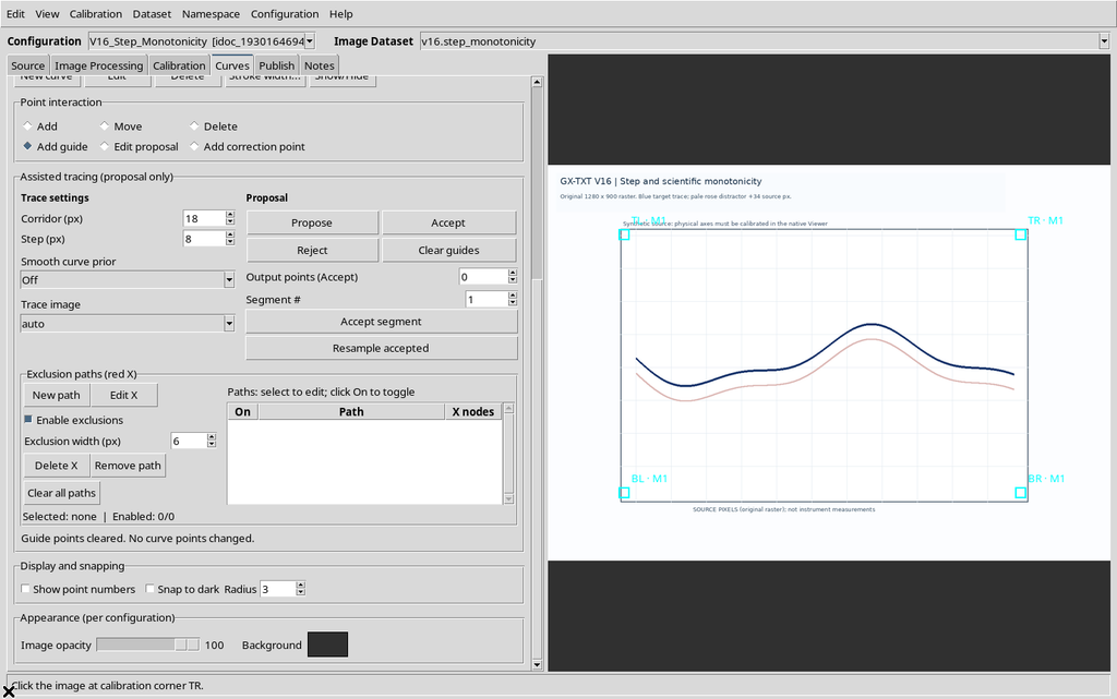
The Clear guides command removes the temporary guides; the scientific points and the source image must not be altered by this operation.
23. Apply, Save and Reopening
The monotonicity criterion belongs to the current configuration, not to an undifferentiated global setting. After Apply, save the configuration with Configuration → Save configuration. If you want to check persistence, close the Viewer normally and reopen it from the current Session.
In the case shown, reopening keeps Monotonic in X / Sort by X, the calibration and the series, while Step returns to 2.0 and the provisional guides are not restored.
This behavior distinguishes the saved parameters of the Interactive Document from the transient panel that drives a single assisted run.
24. Provisional Proposal and Scientific Data
The cyan polyline is a candidate to be checked, not a new Dataset. The numerical values read from the Canvas for the tests in this guide were used to compare the proposed geometry, but were not accepted into a curve or published.
The Assisted trace output points parameter, if used, concerns the number of numerical points wanted at acceptance time, and is distinct from the Step sampling used for the search on the raster. Interpolating a sparse candidate does not recover experimental details that were not recognized in the original proposal.
25. Recommended Workflow
- Check the image, the calibration and the target series.
- Choose the path criterion consistent with the geometry: free, X or Y.
- Place at least two guides, adding more near ambiguous regions.
- Set Corridor and Step in original pixels; start from the default value if there is no reason to change it.
- Press Propose and check the number of points, the segments, the Step message and the course on the raster.
- Compare other Steps when needed; do not infer quality from the number of points alone.
- Use Reject for an inadequate proposal. Point-by-point correction and acceptance are covered in the next chapter, devoted to reviewing the proposal.
26. Summary and Limits to Remember
The Step parameter determines the density of the searched tracing, within 0.5–20 px of the original image. Monotonicity determines how the guides are ordered according to a scientific axis, while simple ordering can also be applied without declaring that the curve is monotonic.
There is no universally optimal Step value: in this example 8 px showed the smallest deviation from the synthetic line, but the outcome depends on the stroke, the raster, the guides, the corridor and the prior. The effects of Smoothness, of excluded regions and of corrections to the proposed points will be illustrated separately, without confusing them with the function of Step.