

Previewing, Comparing and Publishing the Processed Image
Image Processing lets you examine a scientific image after intensity, color and contrast filters have been applied. In the GX-TXT Curve Digitalizer you can compare Original and Processed, navigate the two views, keep a filter pipeline in the configuration and, if the result is satisfactory, publish a new canonical Image Dataset.
It is essential to distinguish four objects: the source image, the filter sequence, the temporary preview and the Dataset that may be published. Curve digitizing always uses the coordinates of the original raster, while the filters change only its appearance.
1. Starting from a Verifiable Original Source
The example figure contains four colored synthetic traces, a grid and slight noise. It measures 1280 × 900 pixels and was loaded into the Viewer as the original Image Dataset.
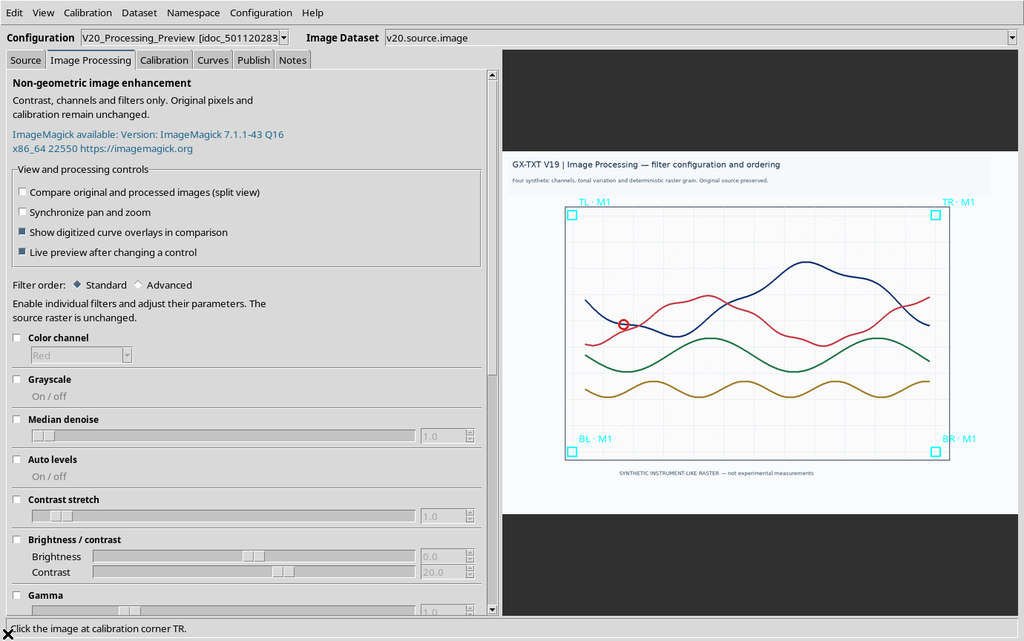
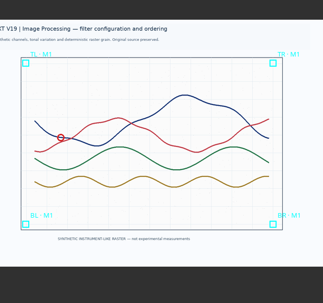
The four-corner calibration maps X to 0–10 s and Y to −20–80 mV. A series also contains a manual point: it will be used to check that pixel operations are not mistaken for changes to the numerical points.
2. Where Apply and the Other Commands Are
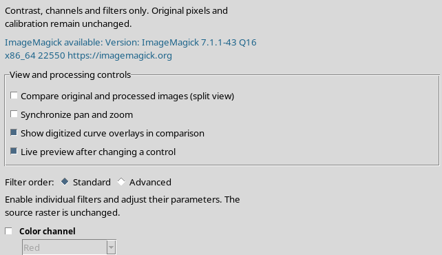
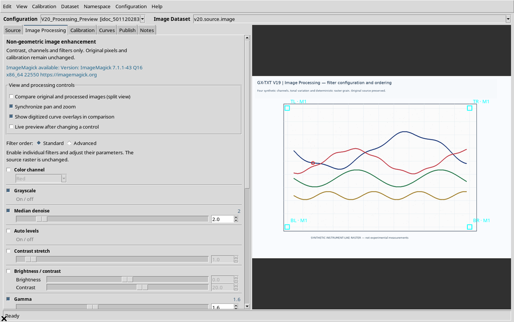
Open Image Processing from the tab bar or from View → Image Processing…. The filter rows are configured on the left side. The Apply processing / Preview command computes the result, while Show processed preview chooses which version to show.
Compare original and processed images (split view), Synchronize pan and zoom and Show digitized curve overlays in comparison are used for visual assessment. Publish image.raster Dataset… is instead a separate choice that creates a new canonical object.
3. Apply Without Active Filters
If no operation is enabled, pressing Apply processing / Preview does not produce a new image. The Viewer reports that there are no operations to apply.
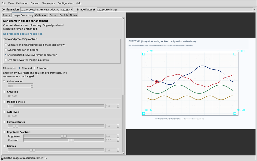
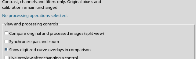
This is the expected behavior: you first need to choose at least one filter with its checkbox.
4. First Preview: Grayscale
Enable Grayscale and, for this example, turn off Live preview after changing a control so that the calculation must be requested explicitly.
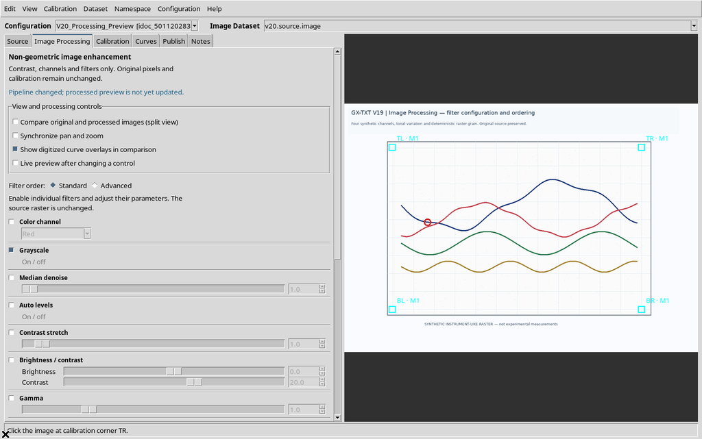
Press Apply processing / Preview. When processing ends, the GUI confirms Ready: 1280 × 900 px; raster geometry unchanged.
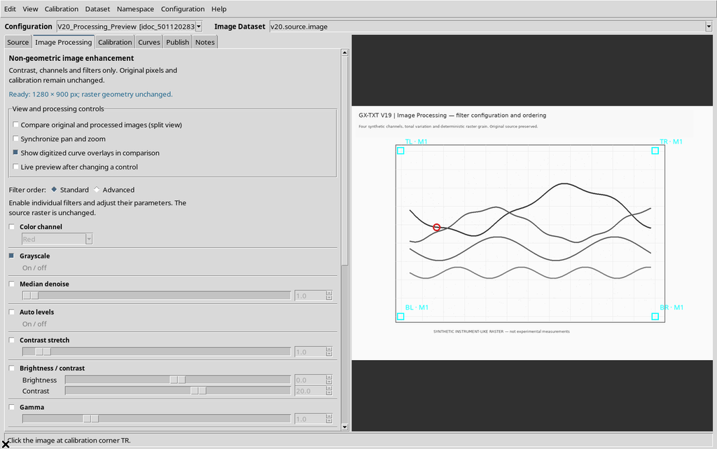
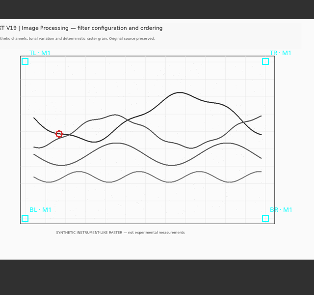
The curves change their tonal rendering, but not their position or size. In particular, conversion to gray can bring two traces closer together that were originally easy to tell apart by color.
5. Original and Processed: Switching Without Deleting
Disabling Show processed preview brings back the original color image.
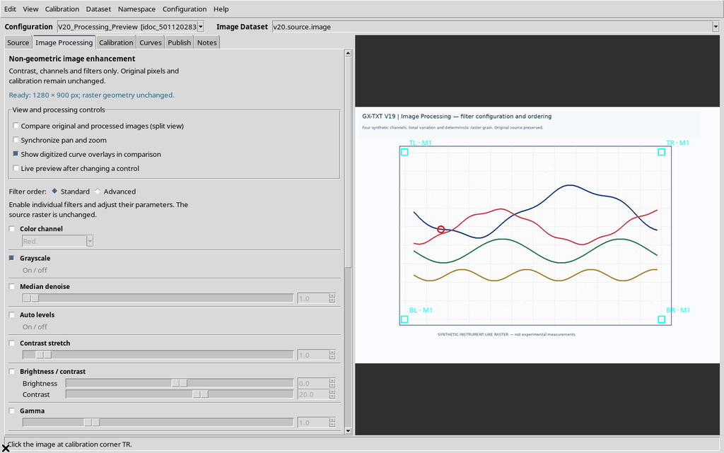
Re-enabling the checkbox shows the processed version again.
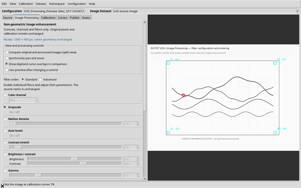
The button does not recreate the original Dataset, does not apply a geometric transformation and does not accept any scientific point. It is a display choice between two images available in the Viewer.
6. Turning On the Side-by-Side View
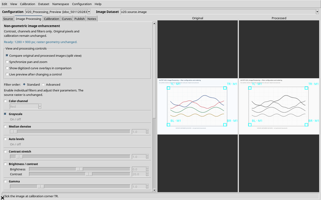
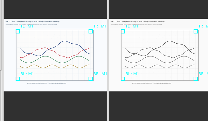
Select Compare original and processed images (split view). The Canvas is split into two panels: Original on the left and Processed on the right.
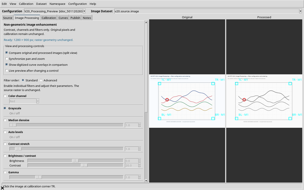
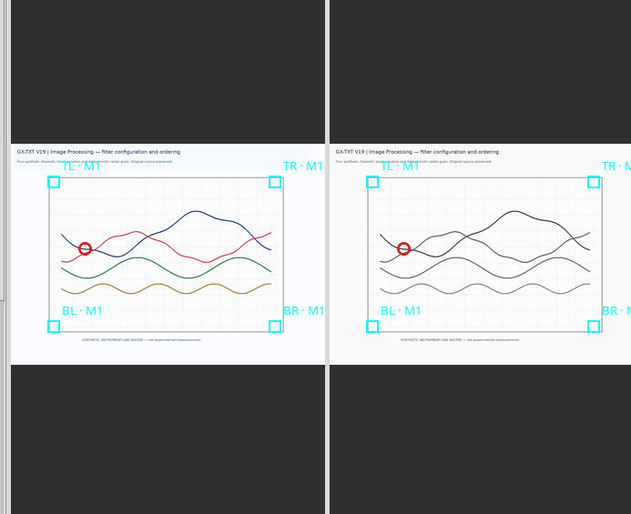
This comparison is particularly useful with several curves, dense grids or faint features: a line made more visible on the right must still be recognizable and consistent in the original on the left.
7. Showing and Hiding the Digitized Points
With Show digitized curve overlays in comparison, the scientific markers are available in both panels. Disabling the function makes the markers disappear from the view.
Re-enabling the command, they become visible again.
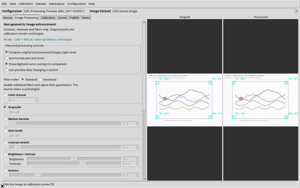
The manual point in the example was not deleted: the function controls the graphic overlay, not the records of the series.
8. Independent Zoom and Pan
With Synchronize pan and zoom disabled, each panel has its own navigation. Use the mouse wheel to zoom into the Original side.
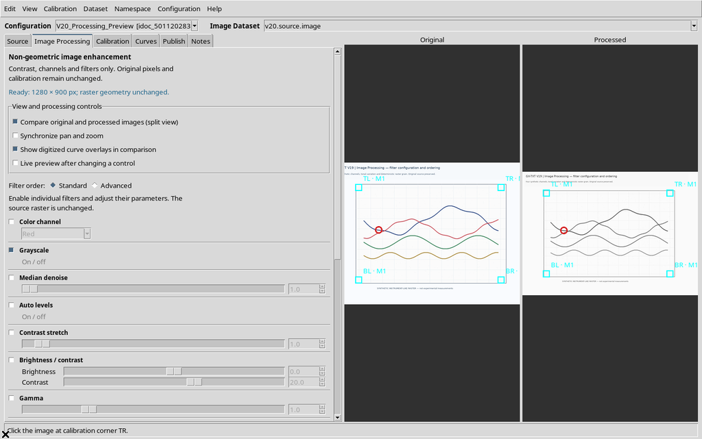
The Processed side keeps its previous level. Likewise, dragging with the right or middle button moves the Original view without dragging the other one.
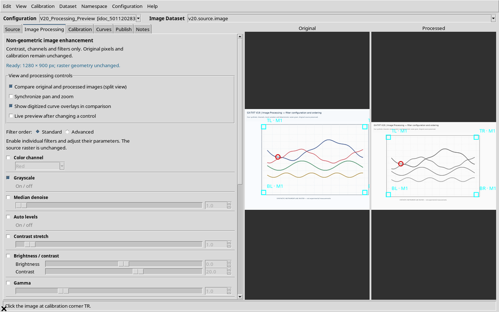
This choice is useful when you want to examine a detail at a different magnification, but makes point-by-point comparison less immediate.
9. Synchronizing the Two Views
Enable Synchronize pan and zoom. The Viewer aligns the two panels on the same position and scale of the source.
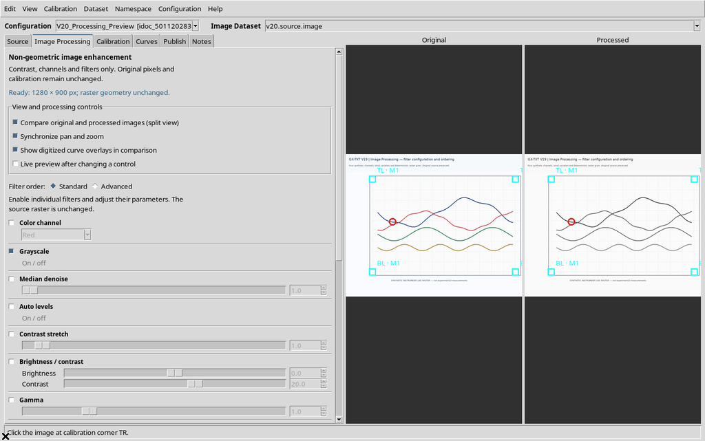
Zooming into the Processed panel now updates Original as well.
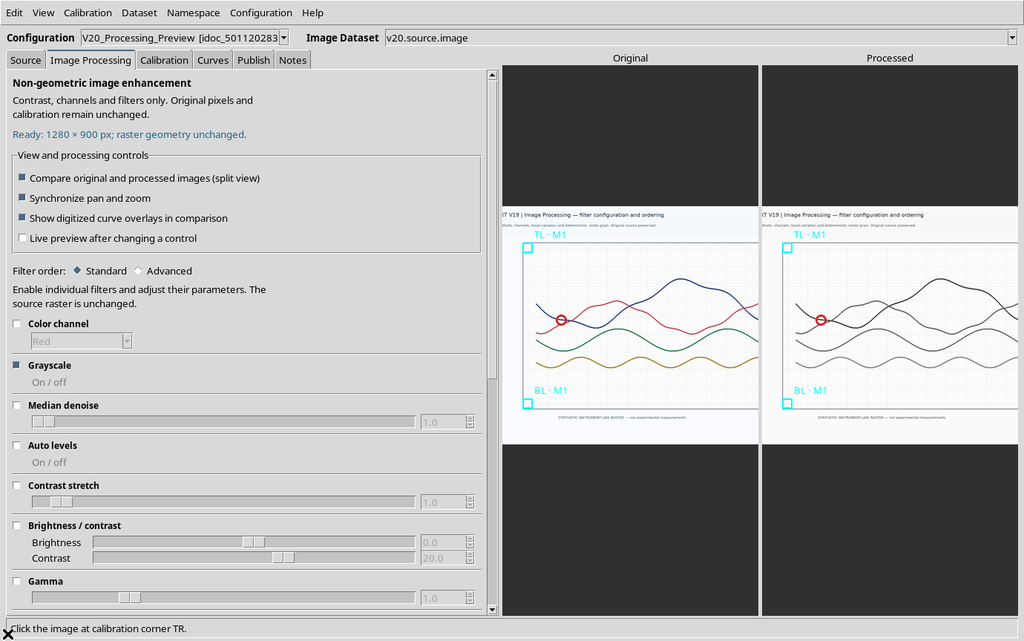
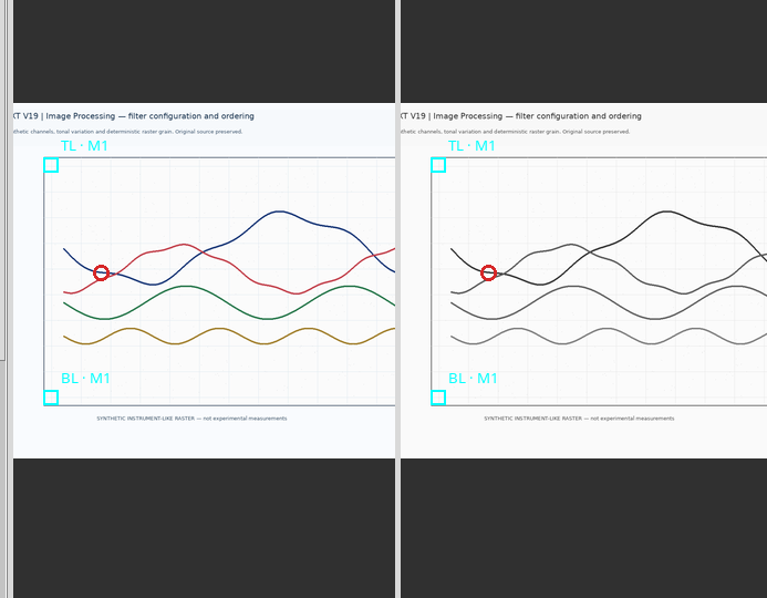
With synchronization active, panning one panel is also reflected in the other.
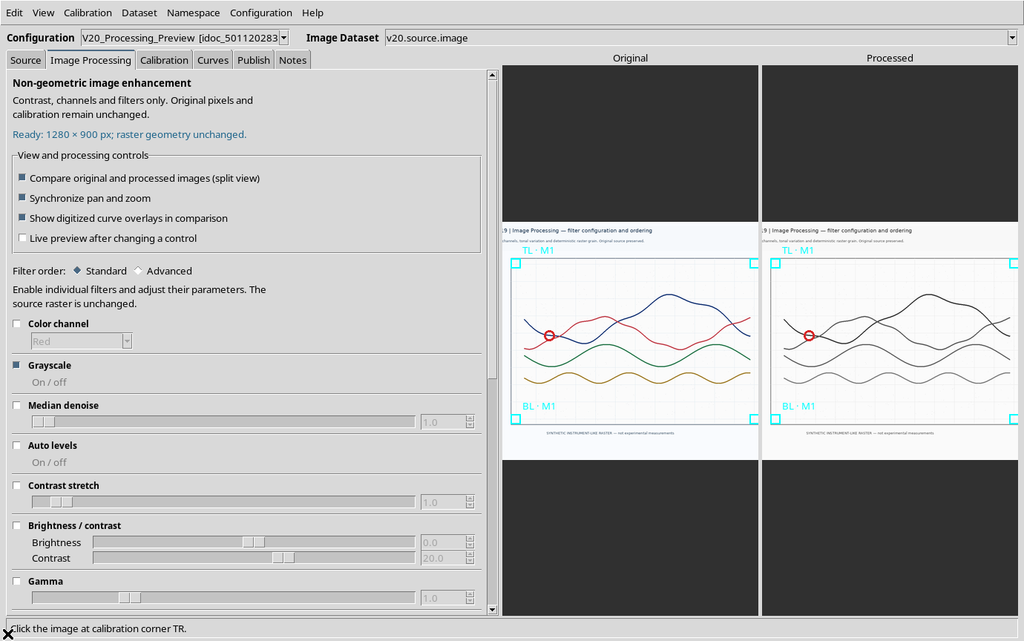
The alignment follows the coordinates of the source raster, not the apparent identity of the lines after processing.
10. Moving the Central Divider
The vertical divider between Original and Processed can be dragged to give more space to one panel.
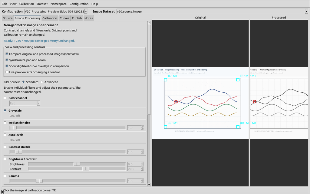
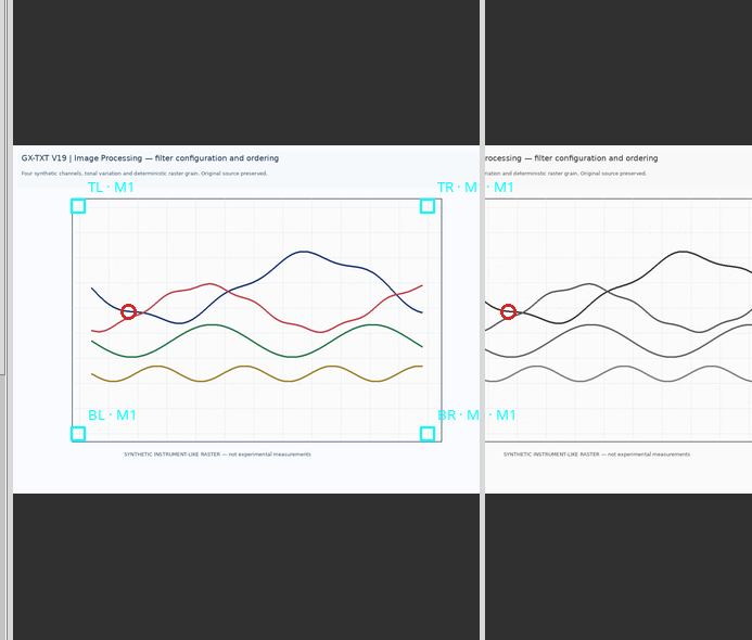
The two areas can therefore have different widths, while synchronization keeps using the same region of the raster. Dividing the space changes neither the size nor the calibration of the images.
11. Back to the Single Canvas and the Curves Tab
Disable Compare original and processed images to return to the single Canvas.
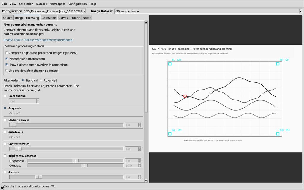
Then open Curves.
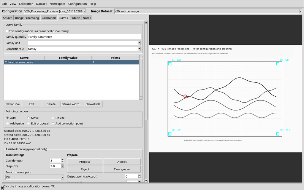
The processed version can stay visible as an aid to digitizing, but the points added from the Curves tab refer to the original coordinates. Going back to Image Processing, the Viewer keeps the single-view choice.
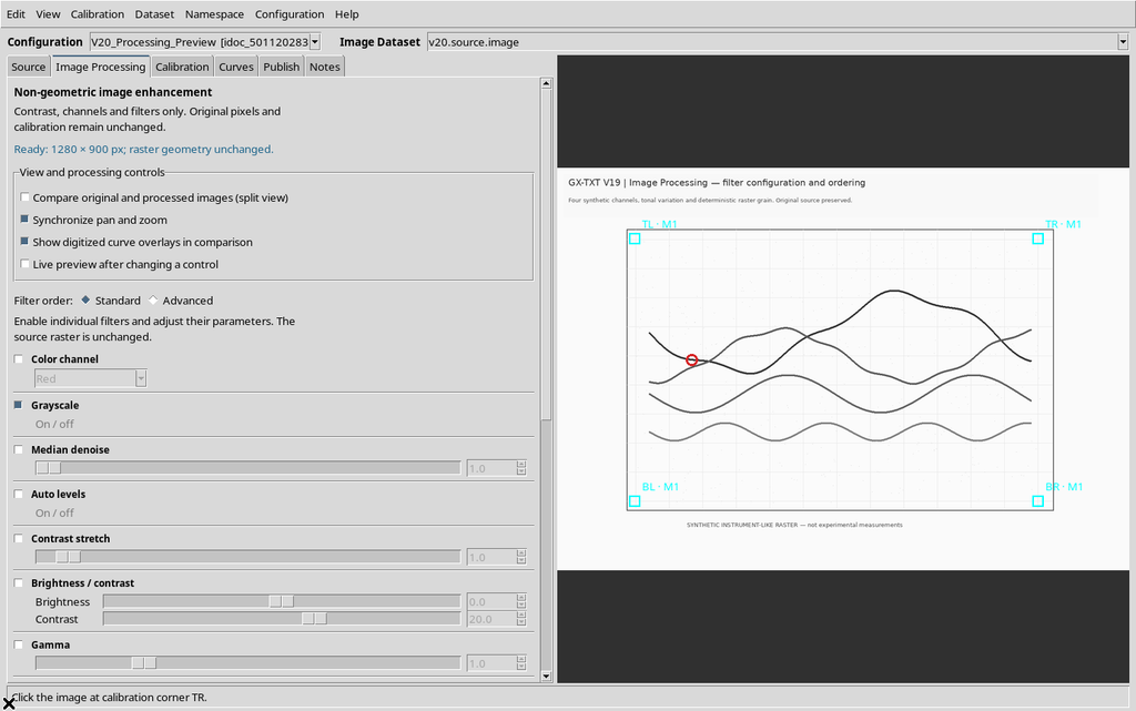
The Image Processing tab must not be used as a point editor: the comparison view neither adds nor deletes scientific points.
12. Live Preview: Automatic Update
Turn Live preview after changing a control back on. Add Gamma to the previous Grayscale operation, setting for example Gamma = 1.45.
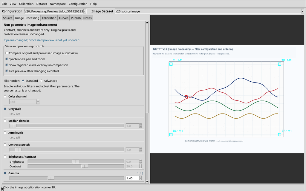
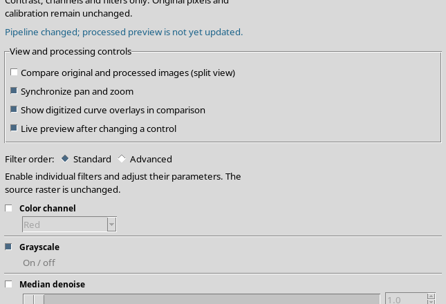
The GUI first reports that the pipeline has changed; then it automatically starts the calculation and shows a new preview consistent with the updated parameters, without having to press Apply again.
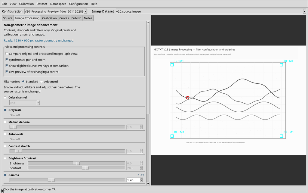
The update is briefly deferred when sliders or fields are changed: this limits unnecessary recalculations during adjustment. Having a preview ready does not mean the result has already been published.
13. Try Automatic Enhancement
The Try automatic enhancement button analyzes the source and proposes a sequence of filters. In the demonstration figure Auto levels and Local contrast (CLAHE) were suggested.
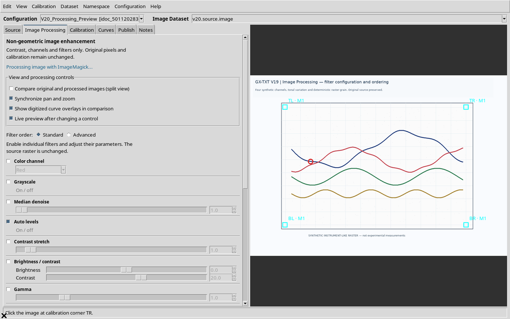
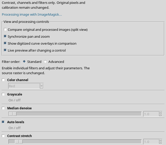
The Viewer can compute the preview of the automatic proposal.
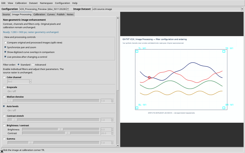
It is a practical suggestion, not a scientific check. It can improve the readability of a line or introduce unwanted effects on faint traces, intersections or edges.
14. Restoring the Previous Pipeline
Restore filters before auto enhancement recovers the sequence used before the automatic suggestion, as long as it remains valid for the current source and configuration.
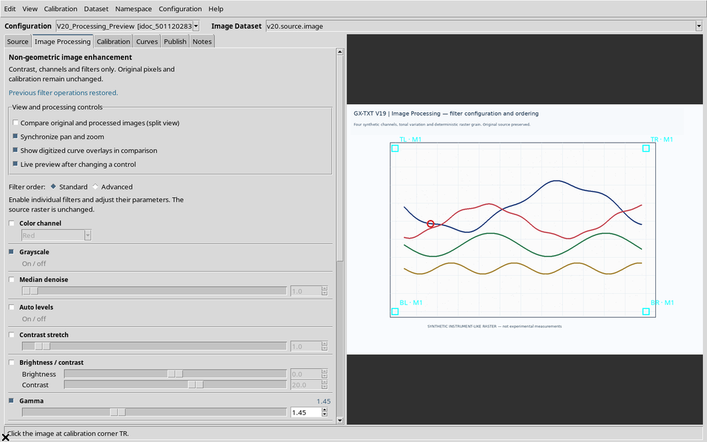
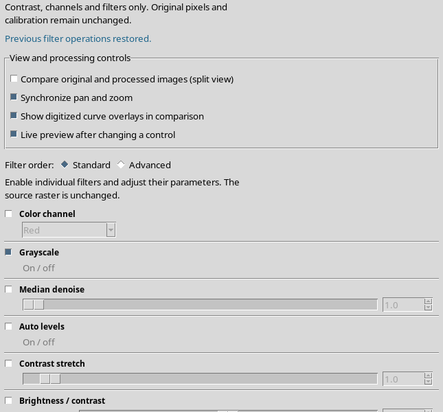
In our case Grayscale and Gamma 1.45 come back. The next preview uses those filters again.
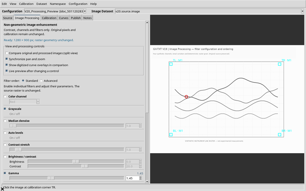
It is advisable to compare both alternatives on the original image before adopting an automatic processing.
15. When a Preview Becomes Out of Date
Suppose Gamma is changed or Median is added after a preview was already ready, with Live preview kept disabled.
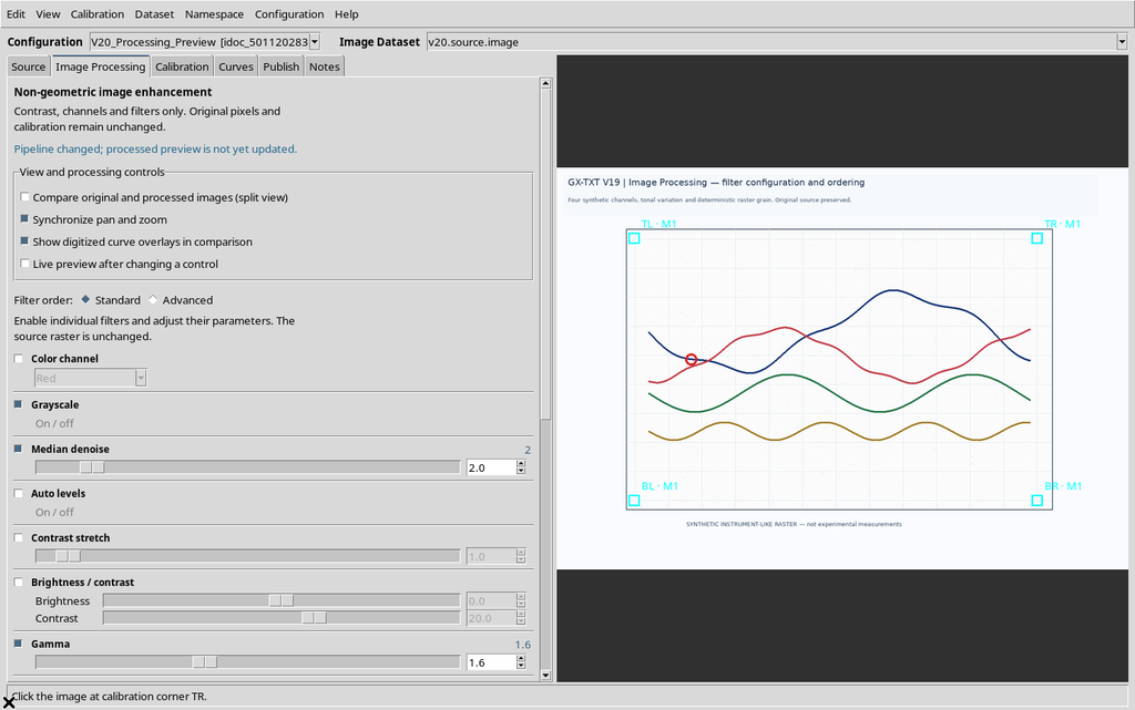
The old visible result does not necessarily represent the new pipeline. If you try to publish it right away, the Viewer blocks the operation and requires a new Apply processing / Preview.
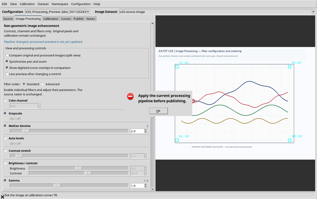
This check avoids associating with a Dataset a list of filters different from the one that actually produced the pixels.
16. Preparing the Pipeline to Publish
For the final example we choose three operations in the Standard sequence:
| Position | Operation | Parameter |
|---|---|---|
| 1 | Grayscale | On |
| 2 | Median denoise | 2 |
| 3 | Gamma | 1.6 |
Press Apply processing / Preview and check the Ready message.
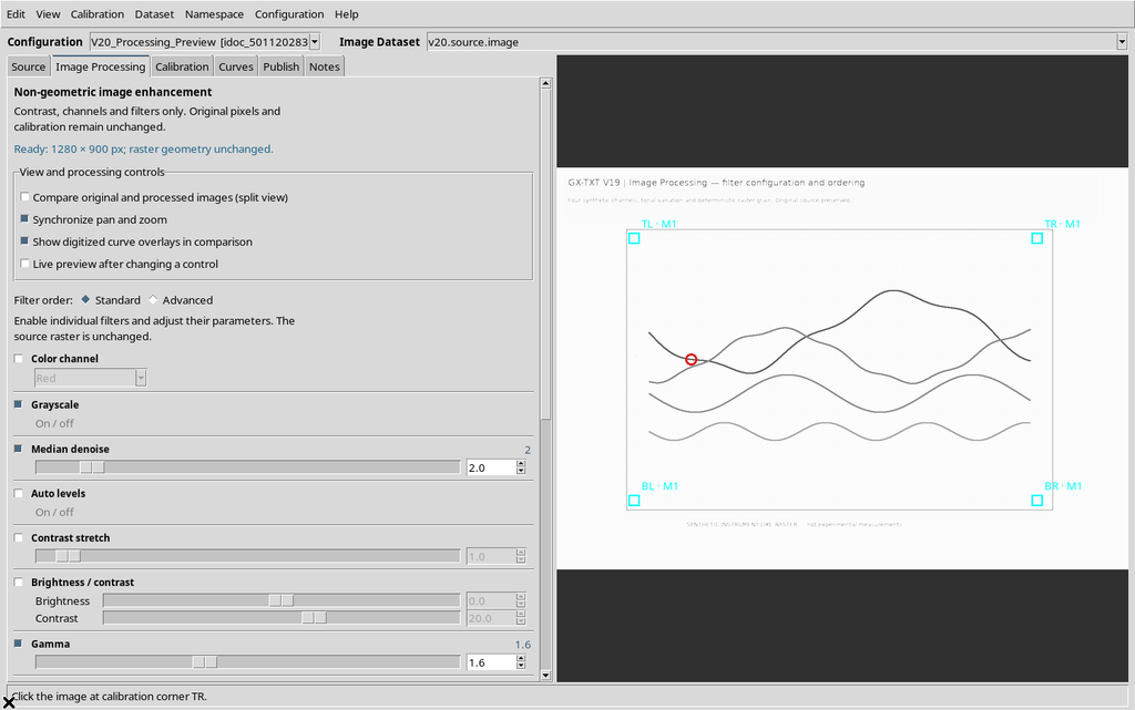
This choice changes colors and intensities but does not resize, rotate, flip or distort the raster.
17. The Output ID Cannot Be the Same as the Source ID
In the Publish processed Image Dataset section, the Image Dataset ID field identifies the new object.
If the same ID as the source is entered and Publish is pressed, an error appears.
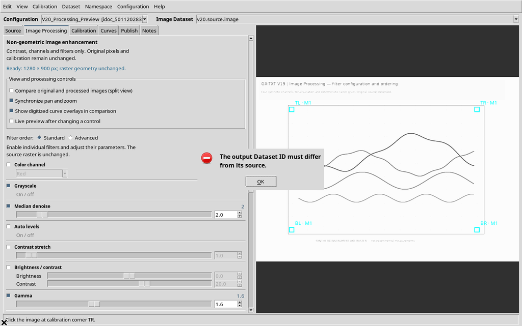
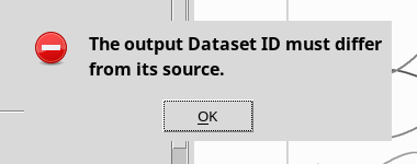
The Viewer thus protects the identity of the original Dataset; the processed image must be published separately.
18. Choosing the ID and Description of the Result
For the example two distinct IDs are used, visible in the Dataset selector:
| Role | Image Dataset ID |
|---|---|
| Starting image | v20.source.image |
| Filtered image | v20.processed.image |
The Image description can state the content, for example Processed V20 analytical color graph. The names are only example identifiers: in your own Session choose clear IDs consistent with the scientific project.
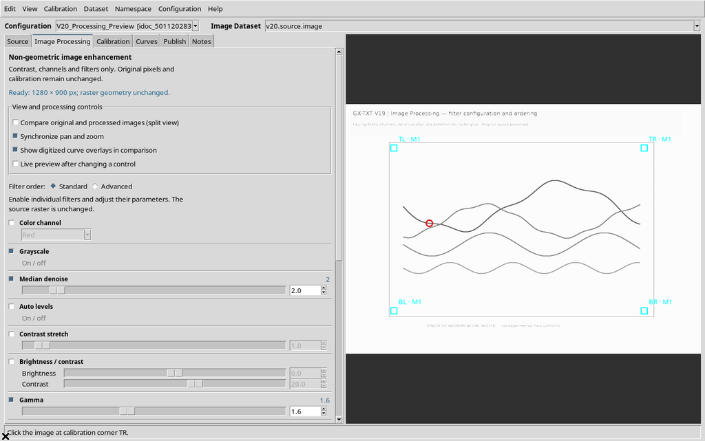
The description accompanies the derived object; the identifier remains its stable canonical identity.
19. Confirming No: Keeping Only the Preview
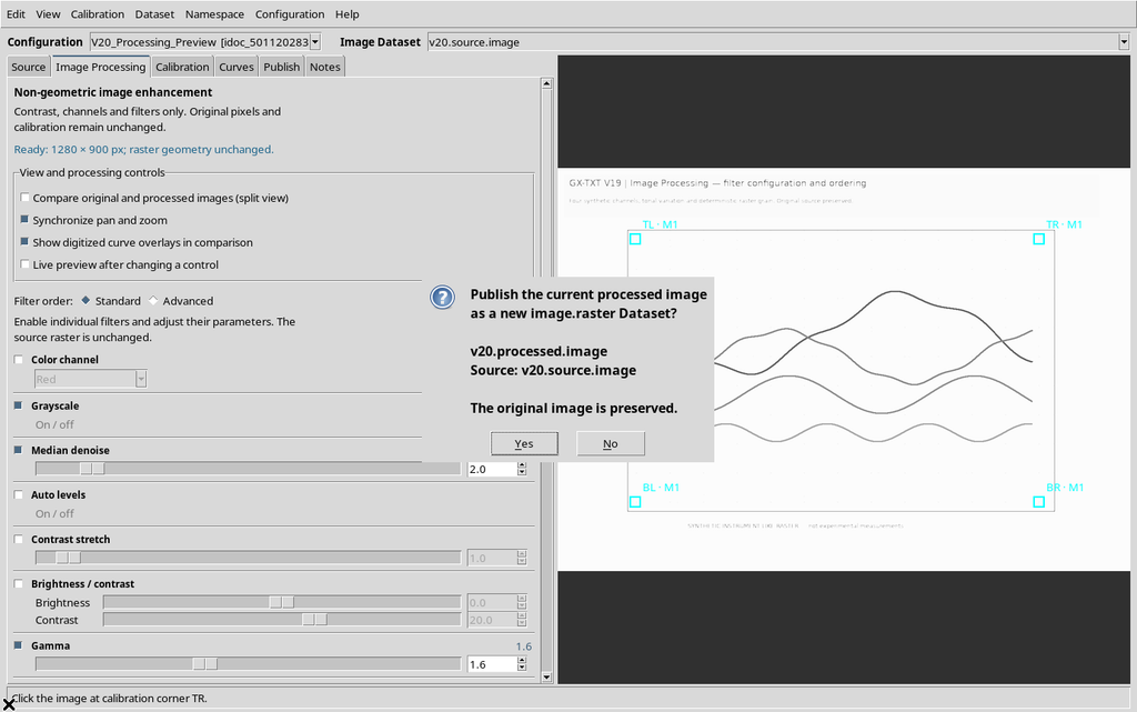
Press Publish image.raster Dataset…. The Viewer shows a confirmation request with the output Dataset and the source used.
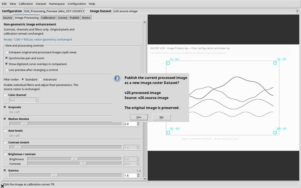
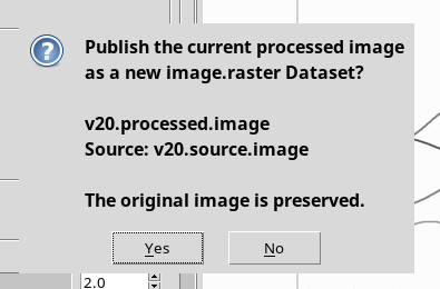
Choosing No, the new Dataset is not created.
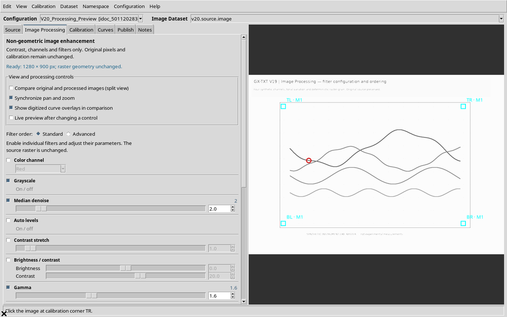
The preview stays available in the Viewer and can still be reviewed or changed. Cancelling the publication does not necessarily cancel the filter settings.
20. Confirming Yes: Publishing a New Image Dataset
Repeating Publish and choosing Yes, the Viewer sends the processed raster to the GX-TXT canonical publishing system.
When the operation ends, the successful publication status appears.
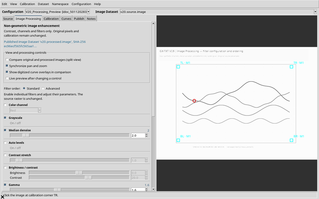
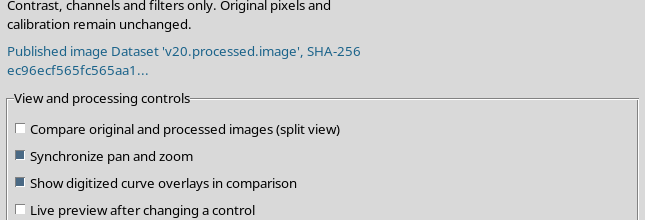
The same Session now contains two Image Datasets: the original and the derived one. Publishing does not change the ID of the first or turn the scientific points of the curve into a separate numerical Dataset.
21. What Is Actually Published
The object created is a standalone image.raster containing the processed raster and a set of provenance metadata. It is not simply the Viewer’s internal preview.
| Feature | Source | Processed Dataset |
|---|---|---|
| Identity | Original | New ID |
| Dimensions | 1280 × 900 | 1280 × 900 |
| Pixel | Original colors | Processed gray levels |
| SHA-256 | Original identifier | Different SHA-256 |
| Geometric calibration | Original reference | Undistorted pixel mapping |
| Numerical traces | Belong to the configuration | Not published with the image |
A processed Dataset can therefore be opened independently, but must not be confused with publishing curves or their uncertainties.
22. Provenance Information Kept
The derived Dataset keeps a manifest including the identifier and SHA-256 of the source, the ImageMagick version, the dimensions, the filter order, the parameters, the unchanged-geometry flag and a fingerprint of the processing.
In the example, the documented order is Grayscale → Median 2 → Gamma 1.6. Changing that order can produce different pixels, even if the individual operations stay the same.
To reconstruct a processing over time you therefore need both the source raster and the exact manifest of the filters, not just the caption of an image.
23. Numerical Check of the Processed Raster
In the example, the pixels of the published Dataset were compared with a second ImageMagick processing run on the same characteristics of the original.
All 1,152,000 pixels underwent at least one change in the RGB channels compared with the source; the result is in grayscale. Repeating the processing with the same parameters produced zero pixel differences from the new Dataset.
This demonstrates the technical reproducibility of this example. It does not mean that the filters increase scientific accuracy, and it is not an estimate of metrological uncertainty.
24. Save, Close and Reopen After Publishing
Save the Viewer configuration with Configuration → Save configuration, close the Viewer normally and reopen it from the same Session.
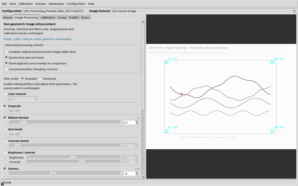
The Grayscale, Median 2 and Gamma 1.6 operations stay recorded; the GUI can regenerate the same preview when ImageMagick is available. The two Datasets keep appearing in the Session catalog.
25. Opening the Processed Dataset in a New Configuration
A published Dataset is not tied exclusively to the preview it came from. You can create a new Curve Digitalizer configuration, choosing the processed version as the Image Dataset.
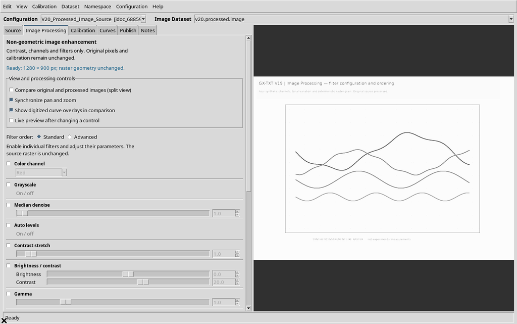
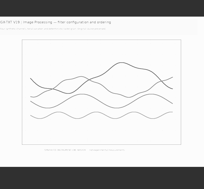
In the new configuration the processed image becomes the source; the scientific points acquired in the original configuration are not copied automatically.
26. Going Back to the Original Configuration
Use the Configuration selector to go back to the document that created the processing.
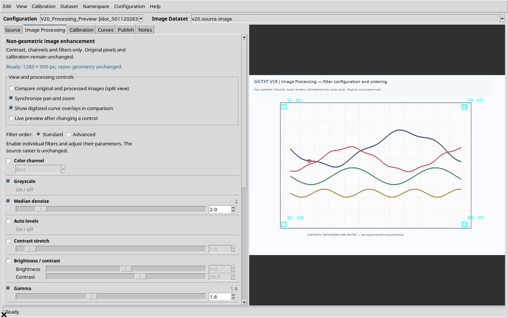

The source becomes the original raster again, with its own calibration and with the manual point already stored. The existence of the derived image neither deletes nor overwrites the initial project.
27. Persistence of the Two Configurations
After another close and reopen, you can still choose the configuration that uses the processed image.
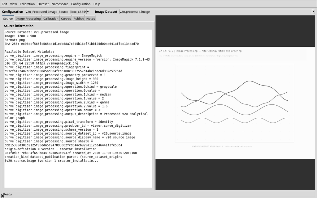
You can then go back to the original one.
The two configurations therefore represent two different workflows: one keeps the direct reference to the source and to the points already acquired; the other lets you start an independent tracing on the filtered Dataset.
28. The Scientific Points Are Not Changed by the Comparison
Comparison, zoom, pan, overlays and preview selection must not be interpreted as commands to add, move or delete points.
In our example, the manual point of the original configuration keeps its identity, pixel coordinates and scientific coordinates throughout processing, publishing and reopening.
Points are edited in the Curves tab with the appropriate commands, not through the Image Processing Canvas.
29. Publishing the Image Does Not Publish the Curves
Publish image.raster Dataset… registers an image with its own metadata. It does not automatically create a Dataset of curve coordinates.
To make the numerical results available, follow the controls of the Curve Digitalizer Publish tab and explicitly choose the series or scientific elements to publish.
The two processes have distinct meanings: one produces a derived raster, the other produces numerical scientific data.
30. Invalid Preview, Delay and Current Source
When the filter, value, order or source changes, the previous preview can become out of date. Before publishing, the Viewer requires the new processing to match the current source and parameters exactly.
With Live preview enabled the recalculation happens automatically, after a short interval; with Live preview disabled you need to press Apply.
The Ready text must be associated with the last pipeline actually computed, not with an old image still present on the Canvas.
31. Appropriate Use of the Automatic Suggestion
Try automatic enhancement can be useful as a starting point for dark scans, uneven contrast or noise. However, do not assume that the proposal is better for every curve.
Always compare the result with Original, especially if a thin line, an intersection or a faint trace risks disappearing.
Restore filters before auto enhancement helps recover the method chosen earlier, without losing control of the experiment.
32. If ImageMagick Is Not Available
The Viewer can still open the image and use the digitizing functions, but it cannot compute a new processed preview without the configured engine.
Check GX-TXT Configuration → Runtime → ImageMagick and the message shown in the Image Processing tab. Do not change the pipeline at random to solve a program availability error.
If processing fails, check the error message before trying again.
33. Watch Out for Bit Depth and Source Characteristics
The pipeline processes a decoded RGB representation of the source image and publishes an RGB PNG image. It is not a system designed to preserve, without transformation, the original depth of every channel of a high-precision acquisition.
For metrological work based on the real pixel intensities, the original Dataset must be kept and used as the authoritative reference.
Contrast, gamma, threshold and noise filters can change the apparent position of edges without changing the coordinate grid.
34. Common Errors and Checks
| Situation | Meaning | Correct action |
|---|---|---|
| No processing operations selected | No active filter | Enable a valid filter |
| Out-of-date preview | The filters changed after the last calculation | Press Apply and wait for Ready |
| ImageMagick unavailable | Engine not configured | Check Runtime |
| Output ID equal to the source | An attempt to reuse a canonical identity | Choose a different ID |
| Publication cancelled with No | No new Dataset registered | Keep checking the preview |
| Automatically suggested operation | Proposed choice, not approved | Compare Original and Processed |
A particularly important check concerns numeric filters: in the version examined, disabling and re-enabling some filters can reset their parameters to the defaults. After a toggle, check the value and the order again before the next Apply.
35. Recommended Workflow
- Load an identified original image and check its calibration.
- Prepare the filters in Standard or Advanced, justifying order and parameters.
- Use Apply processing / Preview or Live preview and wait for completion.
- Compare Original and Processed, possibly with synchronized zoom and pan.
- Check thin lines, intersections, loss of detail and possible artifacts.
- Check the parameters again after any disabling/re-enabling.
- Enter a distinct Image Dataset ID and a meaningful description.
- Confirm Publish image.raster Dataset… only after checking the current version.
- Check that both Datasets exist and that the original source is kept.
- Save the configuration and, if needed, open the processed image in a new document.
36. Summary
Curve Digitalizer keeps image preparation separate from point collection and from the publication of numerical results. Image Processing can provide a more readable version of the graph, while Original keeps the reference to the pixels and the calibration.
Side-by-side comparison, synchronized navigation, filter restoration and publishing confirmations make it possible to keep control of the path from the source image to the derived Dataset.
The decisive choice remains scientific: an image that is easier to trace is not automatically more accurate. Always keep the original and visually check any processing before using the digitized curve in further analyses.