

Stroke Width, Quality Diagnostics and Scientific Control
A curve derived from an image has at least two aspects to distinguish: the position of the numerical points, obtained with the calibration, and the visible thickness of the stroke, a property of the image. The GX-TXT Curve Digitalizer lets you measure the width of the stroke and consult descriptive diagnostics of the curves through the published Datasets.
This guide covers Stroke width, the Quality Schema v2 report and the public APIs that make it possible to read them. None of these tools, on its own, is an estimate of accuracy or of metrological uncertainty.
1. A Curve with a Known Thickness
The example figure contains a dark trace on a light background, a grid and a thinner pink line. The raster measures 1280 × 900 pixels. For the dark trace a nominal thickness of 11 original pixels was set.
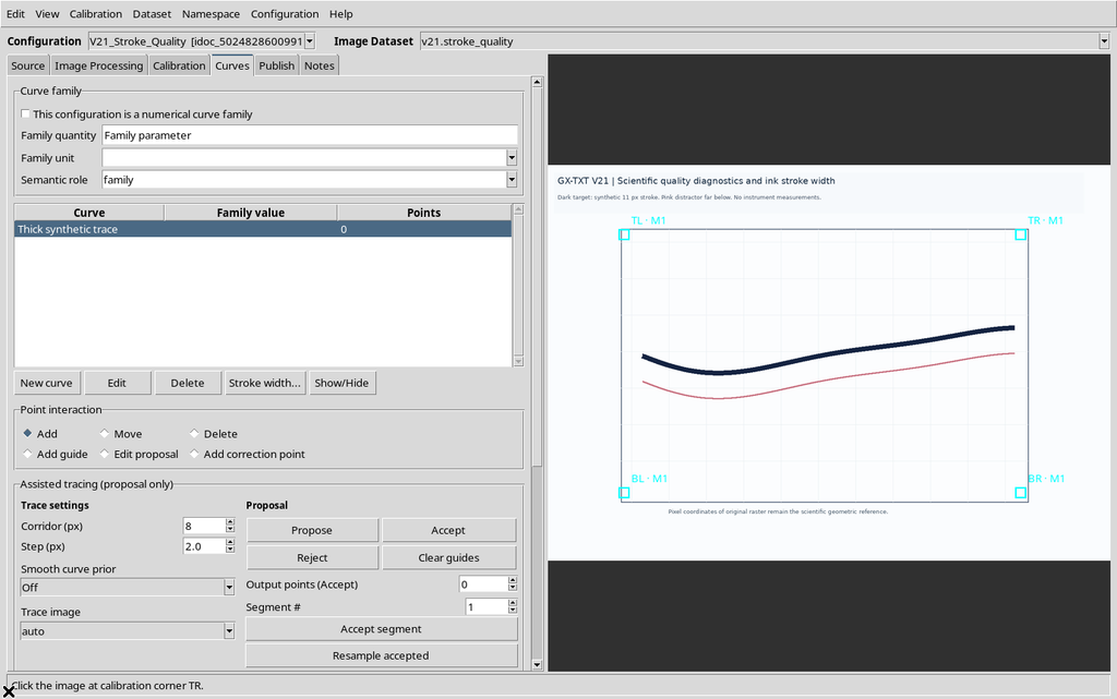
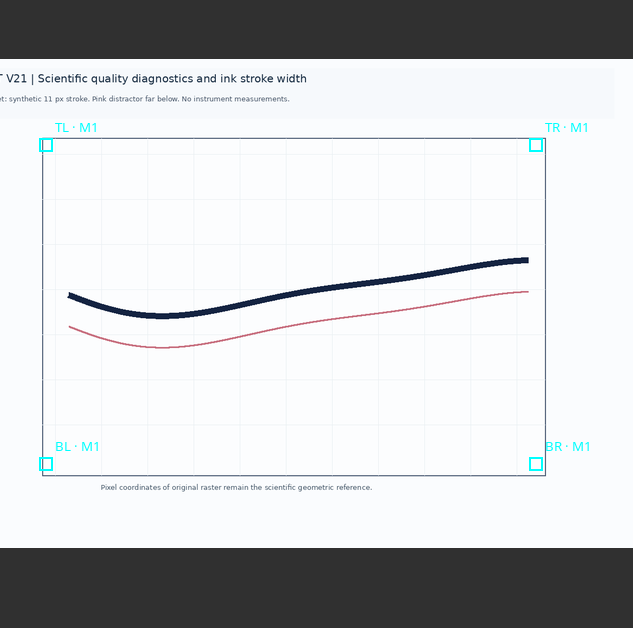
The four-point calibration maps X to 0–10 s and Y to −20–80 mV. Measuring the thickness does not change this transformation. The value of 11 pixels is a geometric property of the teaching figure, not the uncertainty of the Y quantity.
2. Opening Stroke Width
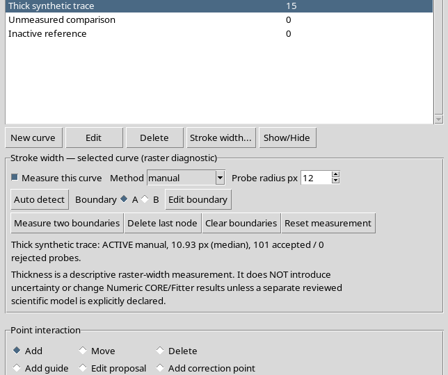
In the Curves tab, select a curve and press Stroke width… to expand the panel. Available are Measure this curve, the automatic / manual method, Probe radius (px), Auto detect, the boundaries A and B and the commands to measure and correct the boundaries.
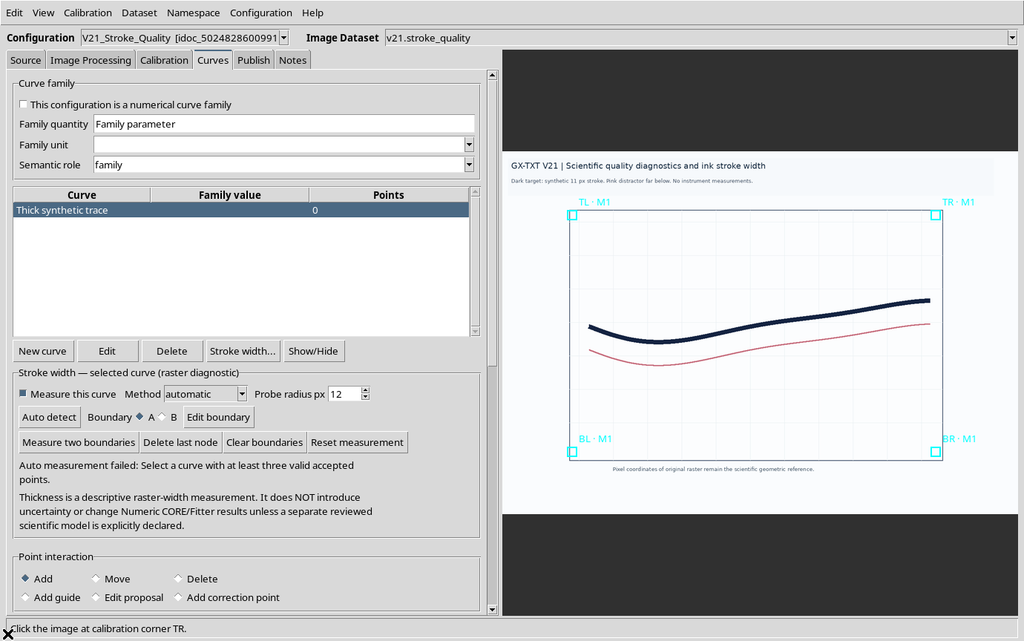
The function starts disabled for the selected curve. Its state is therefore a property of the individual curve, not a value shared by all the series in the configuration.
3. Enabling the Curve Measurement
Select Measure this curve to allow the width to be measured. In automatic mode the sequence of acquired scientific points is used to recognize the local direction of the stroke and look for its edges.
It is not enough for a line to be visible in the raster: the program also needs a numerical path with which to associate the measurement sections.
4. Auto Detect Before There Are at Least Three Points
If you press Auto detect on a curve that is still empty, the Viewer reports that at least three accepted points are needed.
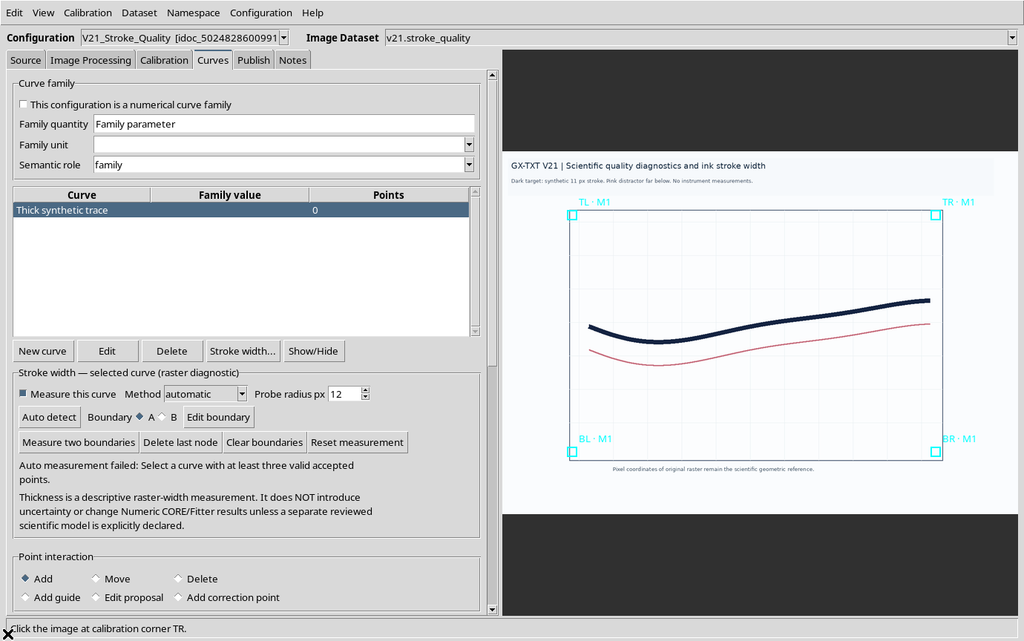
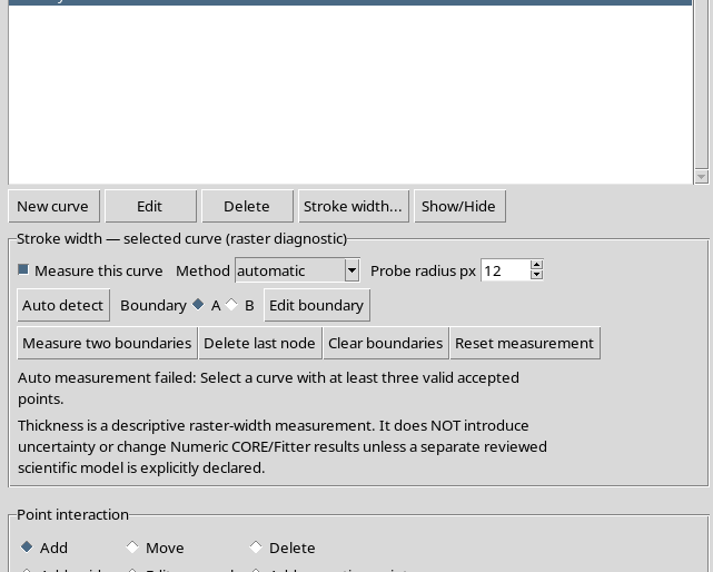
The message prevents an apparently numerical width from being generated without a sufficient trajectory. Add scientific points with the ordinary tools of the Curves tab and repeat the command.
5. The First Measurement After Three Points
Initially three points were placed on the dark line. A first automatic estimate is possible, but the number of available sections is small.
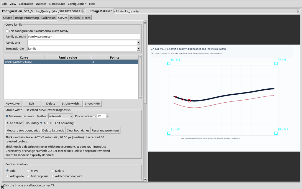
A result built on a single transverse sample cannot describe how the width varies along the whole curve. A more representative check needs points spread over the regions to be examined.
6. Completing the Reference Digitization
For the comparison, up to 15 manual points are added, ordered along the dark line. They form 14 consecutive segments of the scientific path.
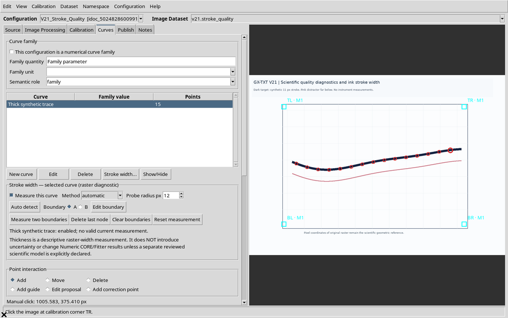
The points keep their original pixel coordinates and calibrated X/Y coordinates. The width of the stroke will be analyzed separately from these positions.
7. Probe Radius: When the Radius Is Too Small
The Probe radius (px) control sets how far from the curve the algorithm looks for the edges of the stroke in the original raster.
With Probe radius = 2 px, the dark stroke in the example is too thick: Auto detect finds no reliable cross-sections.
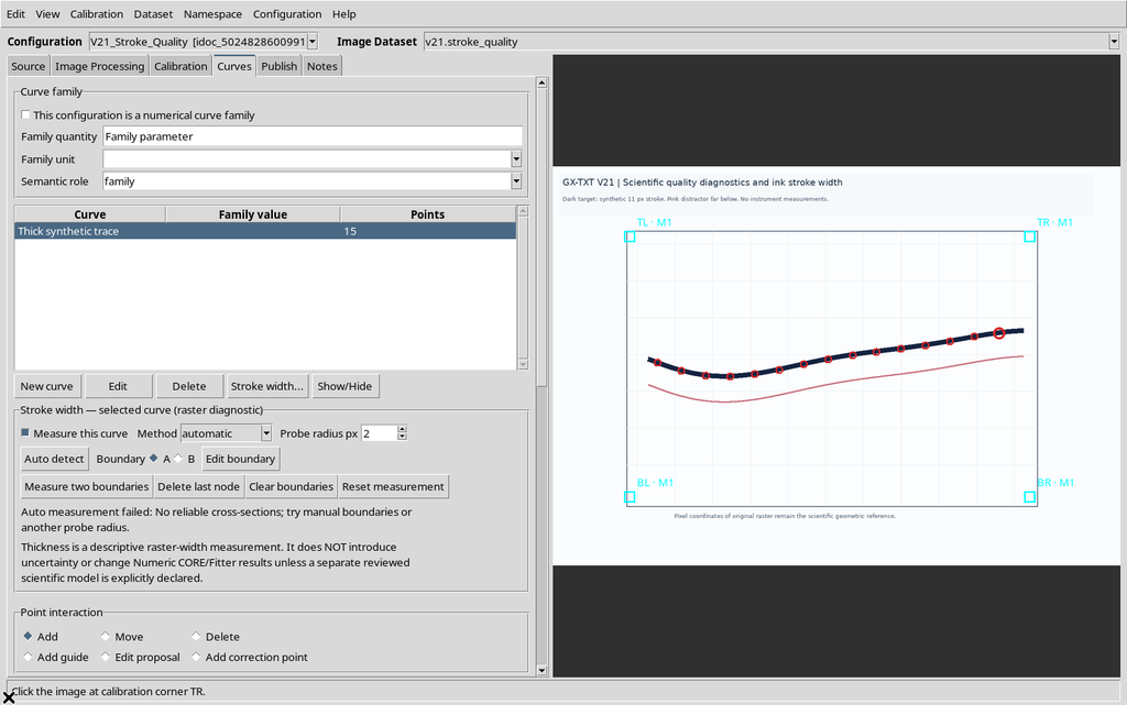
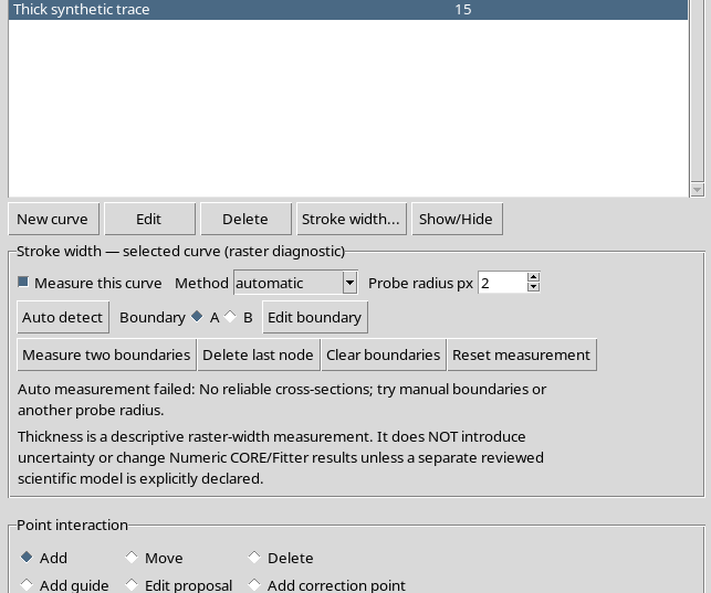
The program suggests changing the radius or using manual boundaries. The limit is expressed neither in physical axis units nor in pixels of the magnified Canvas.
8. Auto Detect with an Adequate Radius
Setting Probe radius to 12 px, Auto detect manages to identify the thickness of the trace along the acquired points.
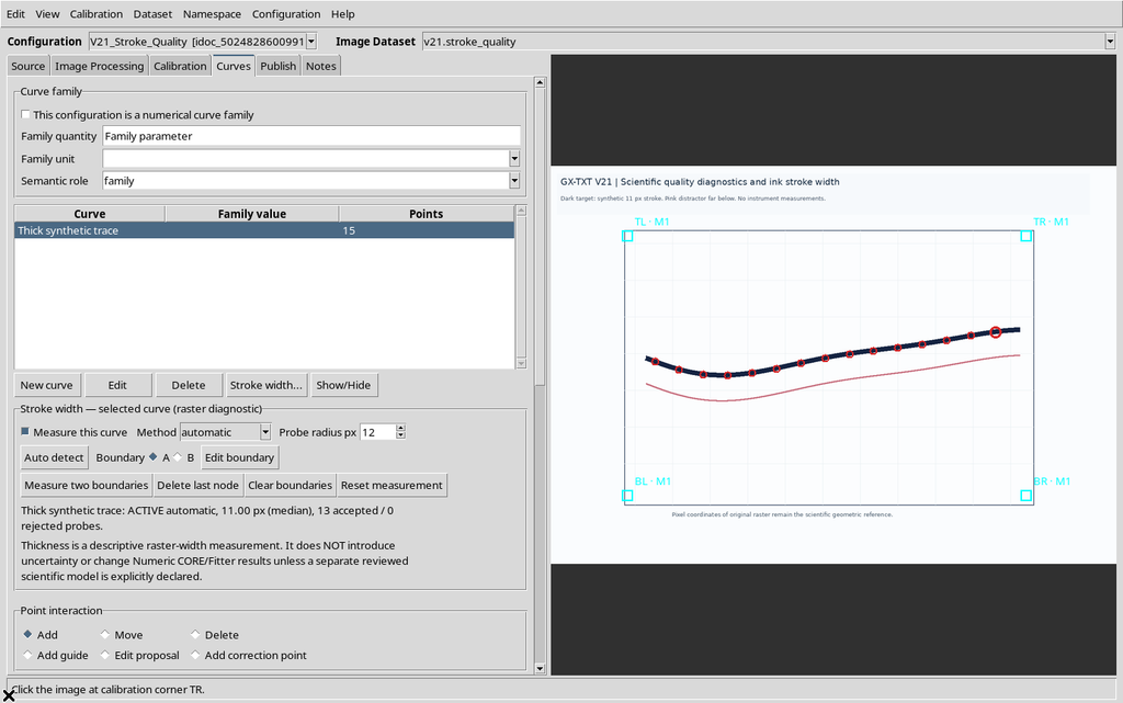
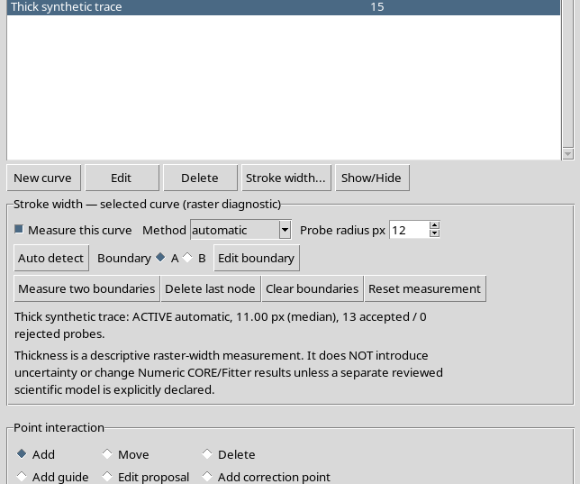
The result in the example is:
| Diagnostic | Value |
|---|---|
| Median width | 11.0 px |
| Minimum | 10.0 px |
| Maximum | 11.5 px |
| Interquartile range | 0.5 px |
| Accepted sections | 13 |
| Rejected sections | 0 |
The median value agrees with the nominal 11 px of the synthetic line. However, the result refers exclusively to the geometry of the stroke in the image.
9. How to Interpret the Thickness Statistics
The median summarizes the thickness of several sections. The minimum and maximum describe the extreme values observed; the IQR measures the spread of the central 50% of the values.
These numbers can help to tell a uniform stroke apart from a line with variable thickness, smudges or confused areas. They must not be interpreted automatically as standard uncertainties, confidence intervals or calibration errors.
10. Choosing Manual Mode
If the stroke is complex, low in contrast or easily confused with other lines, select the manual method. In this case the operator explicitly indicates two boundaries, one for each edge of the line.
Pressing Measure two boundaries before drawing valid boundaries, the Viewer returns no usable result.
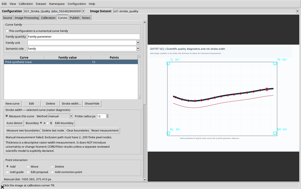
Each boundary needs at least two nodes. The boundary splines are not numerical curves of the publication: they are geometric references for measuring the thickness.
11. Drawing Boundary A
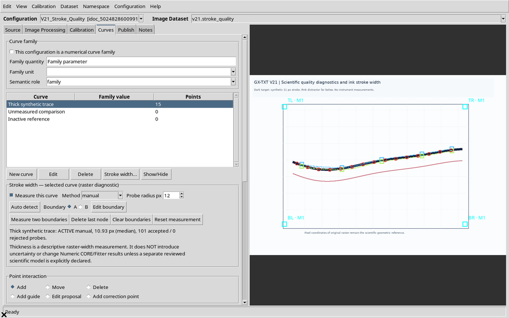
Select A and use Edit boundary. Click along the first edge of the dark stroke. In the test five nodes were placed, shown by cyan markers.
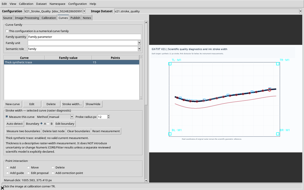
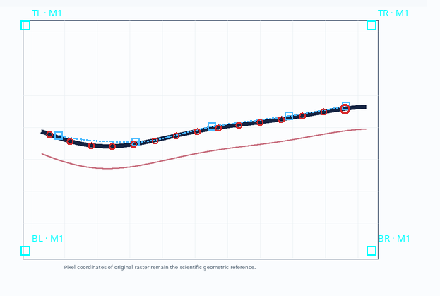
The nodes describe an approximate boundary line. It is advisable to spread them over the stretches where the direction or shape of the stroke changes.
12. Drawing Boundary B
Select B and repeat the procedure along the opposite edge of the line. This boundary also contains five nodes.
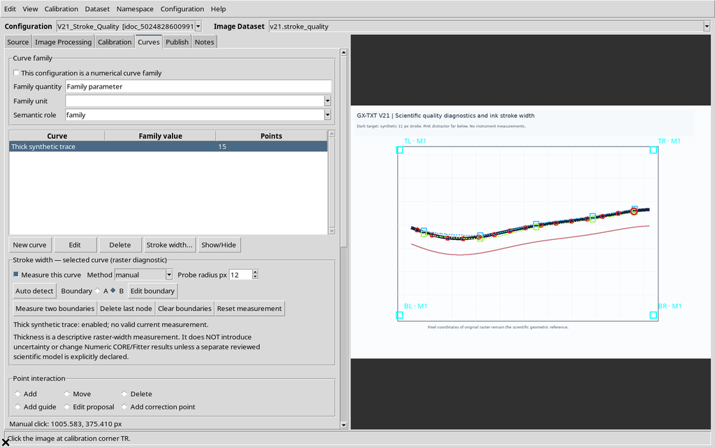
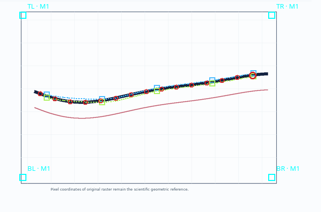
The image thus shows two distinct paths around the original stroke. If the boundaries cross or are badly placed, the result will not represent the width correctly.
13. Measure Two Boundaries
Pressing Measure two boundaries, the Viewer computes the distance between the two boundaries at several positions along their common extent.
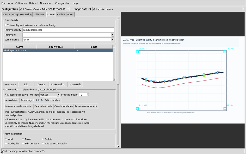
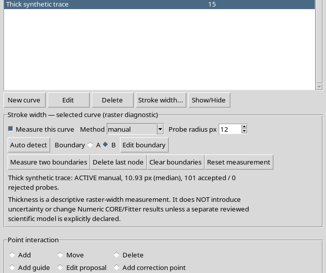
In the example the median width is 10.93 original pixels. The number shown is consistent with the nominal 11 px line. The calculation used 101 interpolated sections between the two splines, not 101 independent experiments.
14. Comparing Automatic and Manual Measurement
| Method | Median thickness | Sections used |
|---|---|---|
| Automatic, radius 12 | 11.00 px | 13 |
| Manual, Boundary A/B | 10.93 px | 101 |
The closeness of the two values is a result of this synthetic graph. The automatic measurement looks for edges in the raster; the manual measurement depends on the boundaries drawn by the operator.
No scientific standard deviation must be derived from the difference between 11.00 and 10.93 px. The two procedures share the source, the geometry and possible distortions.
15. Moving a Node and Invalidating the Previous Result
With Edit boundary, a node of B can be dragged to another position. After the change, the width computed earlier no longer matches the current boundaries.
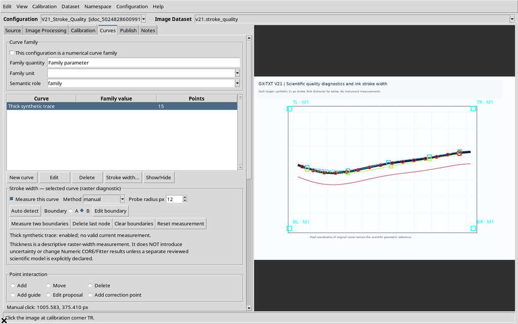
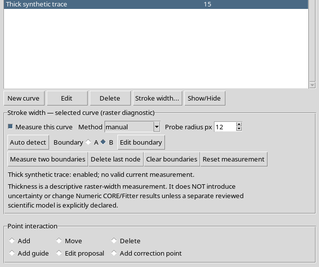
The program marks the result to be updated instead of keeping a number that could look valid. The operator can recompute the thickness or undo the change.
16. Undo and Redo of a Drag
Edit → Undo returns the node to its previous position and restores the measurement that was valid for that geometry.
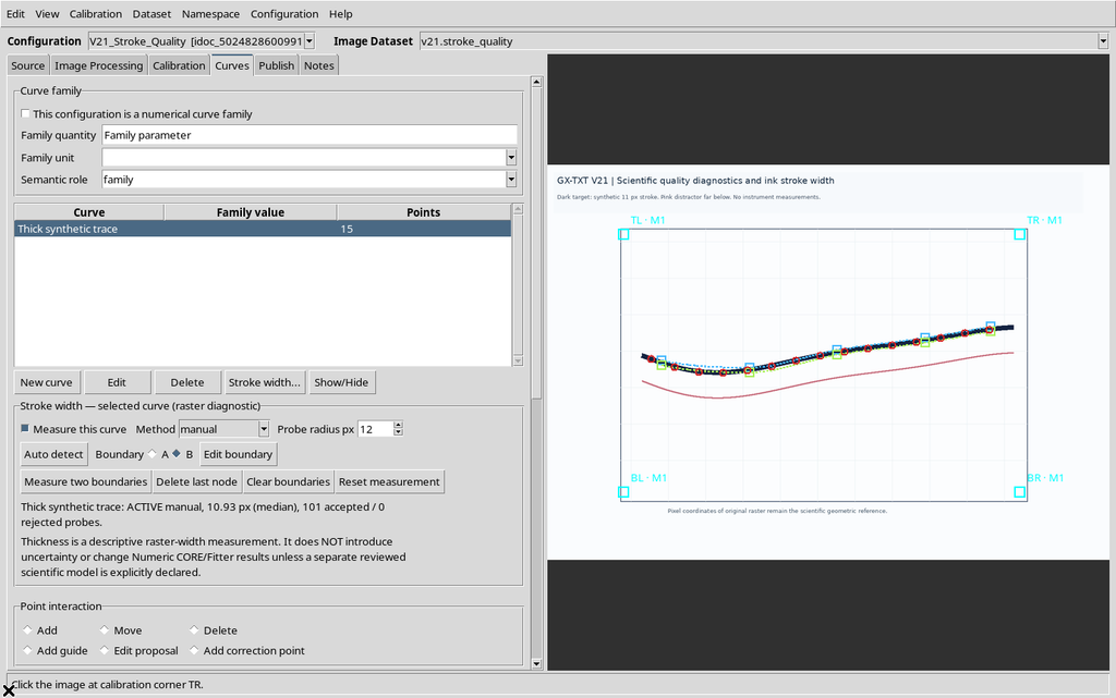
With Redo the move is reapplied, with a new invalidation of the result. The history therefore distinguishes the boundary coordinates from the associated measurement.
17. Delete Last Node
The Delete last node command removes the last node of the selected boundary.
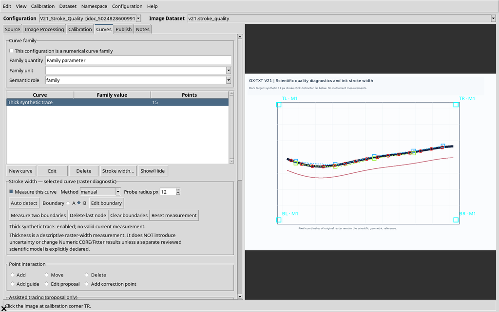
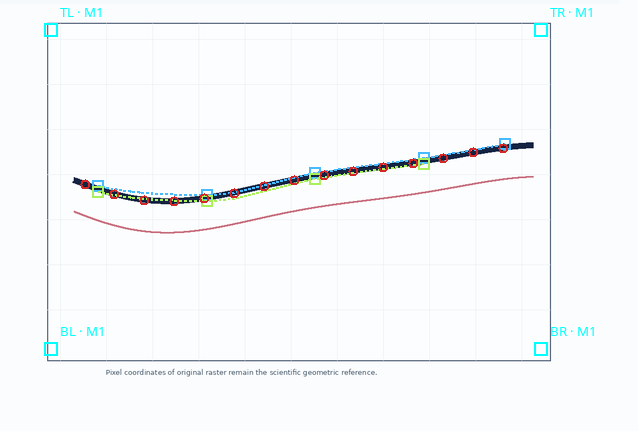
In the example B goes from five to four nodes. Undo recovers the fifth node and the previous geometry. Redo can repeat the deletion, without touching the scientific points of the curve.
18. Clear Boundaries and Restoring
Clear boundaries deletes the two manual paths, leaving the raster and the series of points intact.
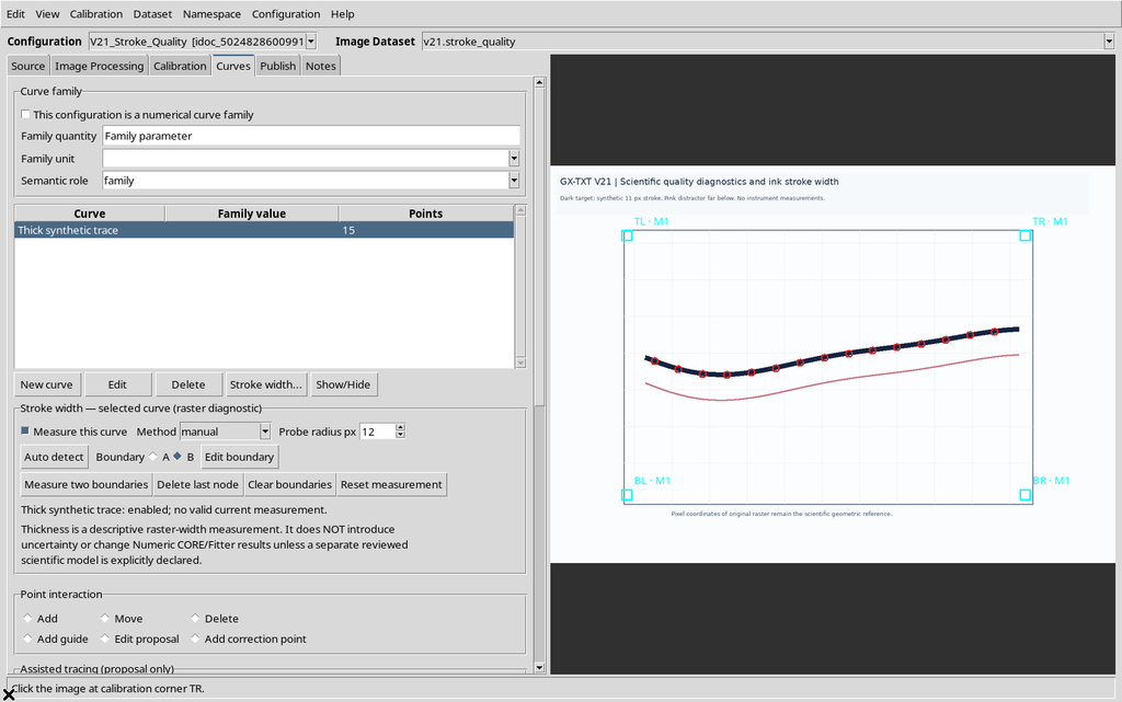
With Undo both A and B are restored.
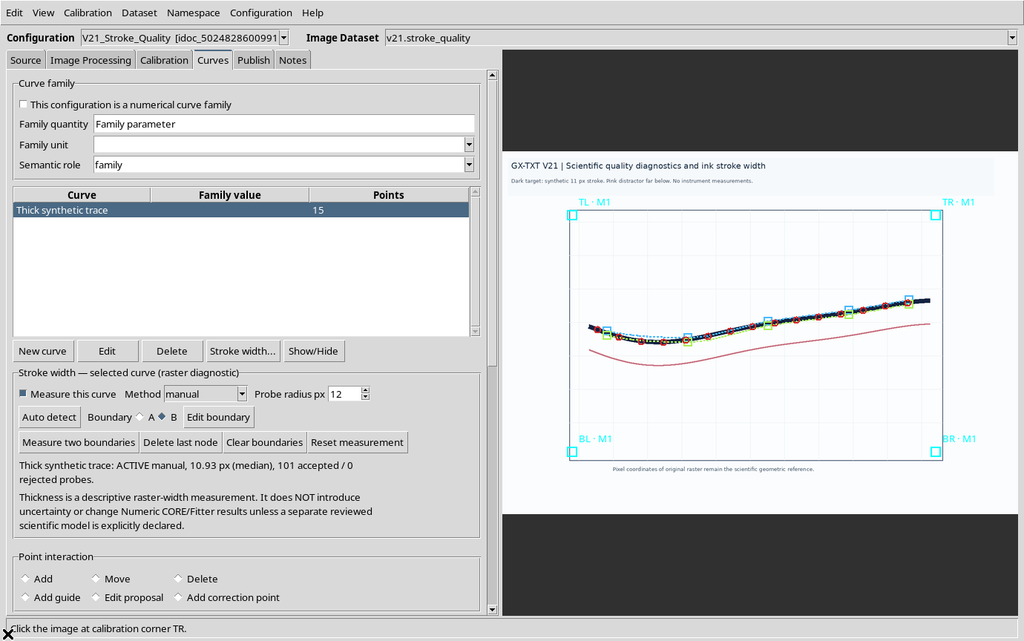
The associated measurement becomes valid again when the history rebuilds exactly the previous geometry. It is still wise to check the boundaries visually after a restore.
19. Reset Measurement Is Different from Clear Boundaries
Reset measurement returns the Stroke width function of the curve to its initial state, inactive.
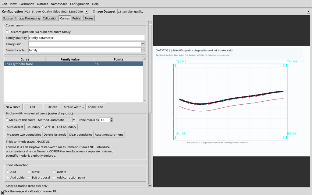
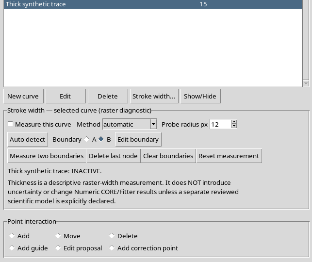
Undo can recover the previous measurement and boundaries.
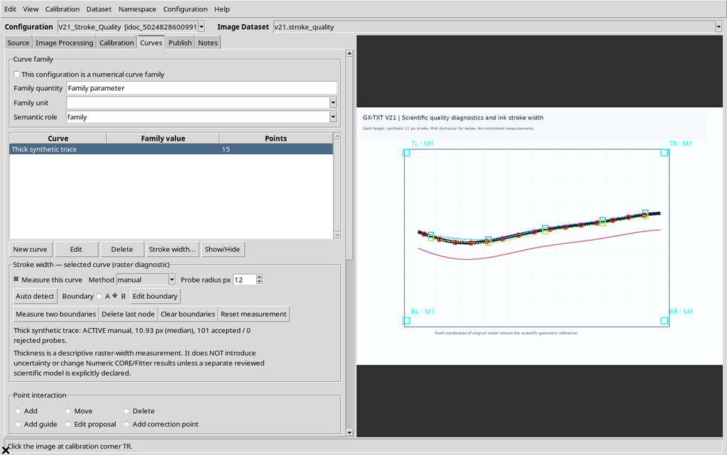
A reset must not be confused with deleting the points of the series, with the Reject command of tracing proposals or with publishing a Dataset.
20. Expanding and Collapsing the Panel
Stroke width… lets you open or close the editor without altering the results.
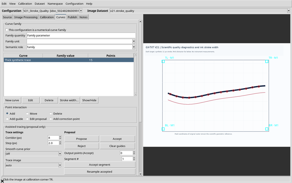
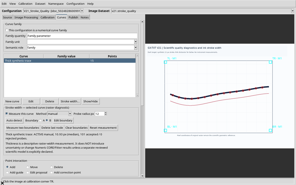
The valid value stays associated with the curve even when the panel is hidden; closing it is only a change in the layout of the controls.
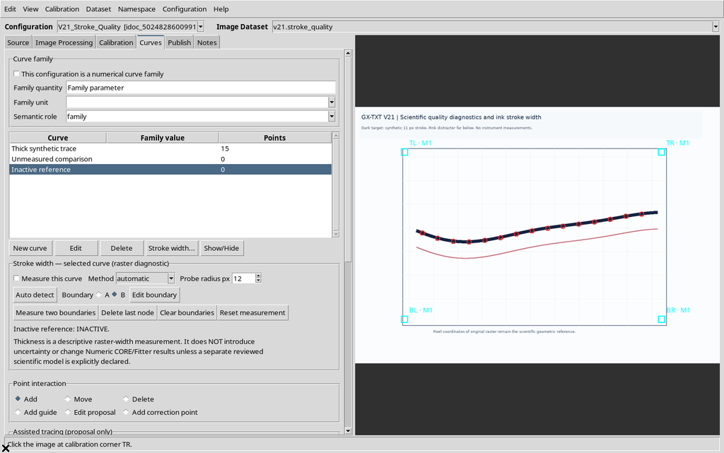
21. Three Curves and Three Distinct States
To check the meaning of the states, we consider three independent curves in the same configuration.
The second is created without points: initially it has no measurement.
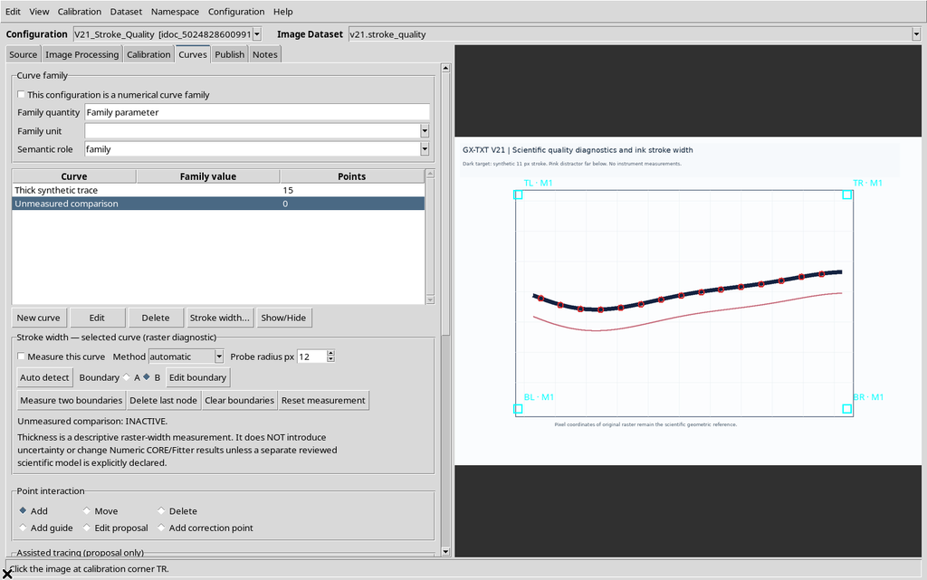
Enabling the calculation on this empty curve, the result stays unavailable.
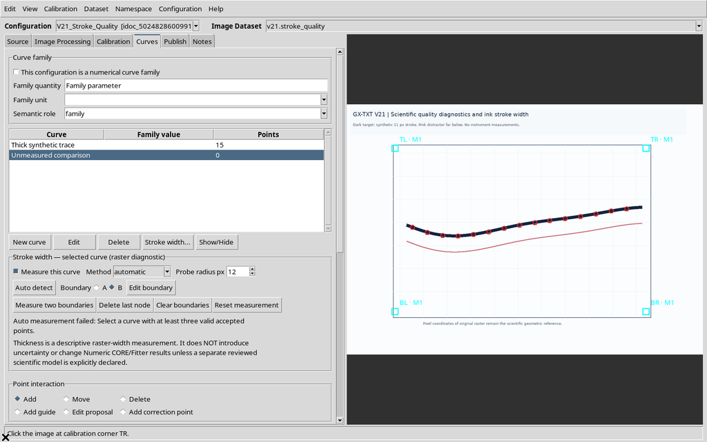
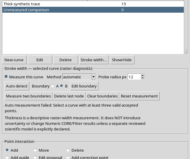
A third curve, on which Stroke width is not enabled, stays inactive instead.
Going back to the first curve, its valid manual measurement reappears.
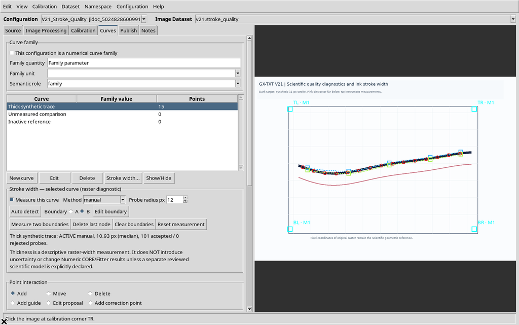
These states are not interchangeable: inactive means not requested, unavailable means requested but not computable, measured indicates a valid result for the current geometry.
22. The Summary in Calibration
The Calibration tab has a Raster stroke width — selected curve section showing the state of the active curve.
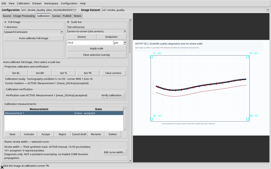
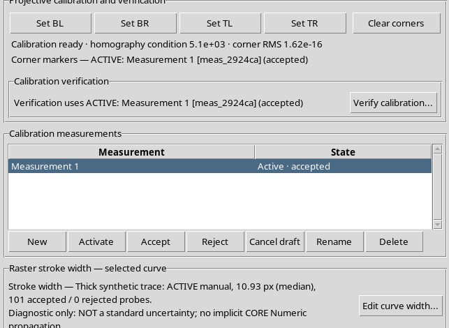
The Viewer explicitly states that this is a descriptive diagnostic, not a standard uncertainty. The distinction is essential so as not to give a statistical meaning to a graphic feature.
Selecting an inactive curve gives a summary consistent with that state.
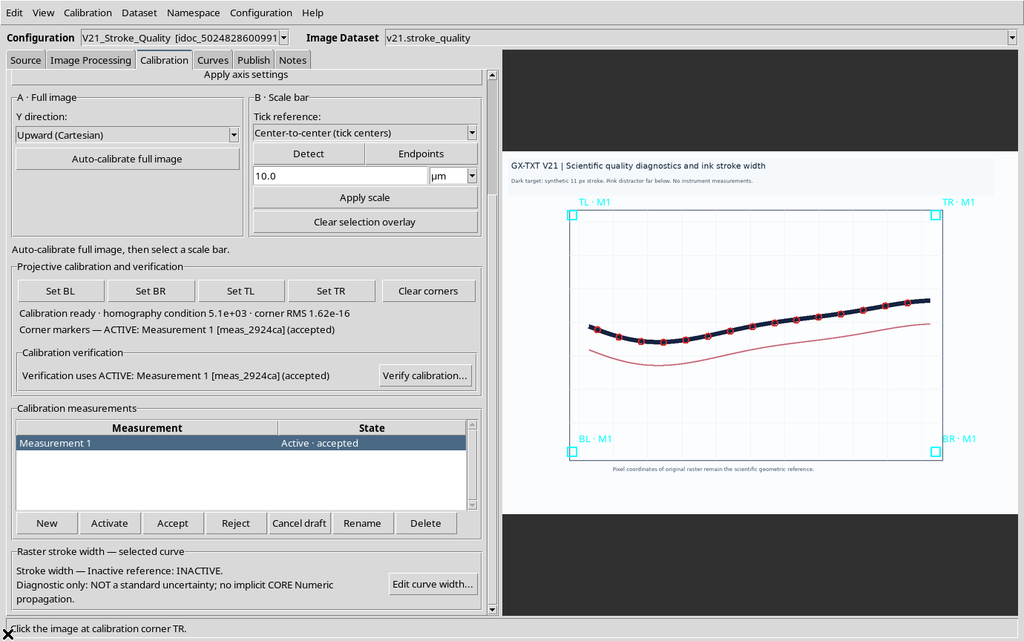
From Edit curve width… you can go back to the editor in the Curves tab.
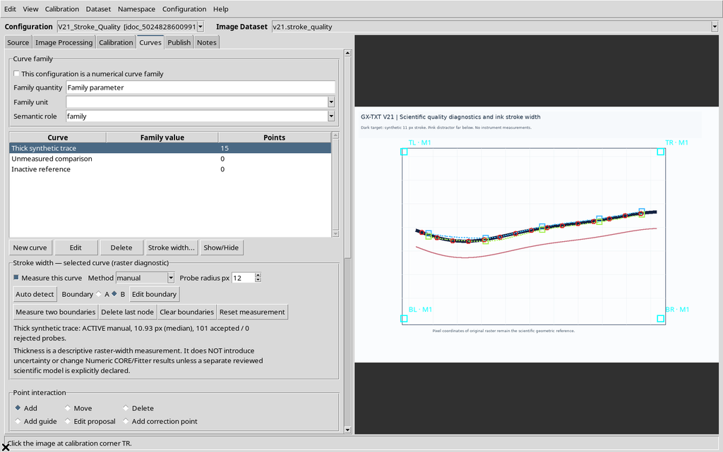
23. Preparing the Scientific Publication
To make the scientific points available in a stable way, open Publish, choose the accepted calibrations and set the identity of the numerical Dataset.
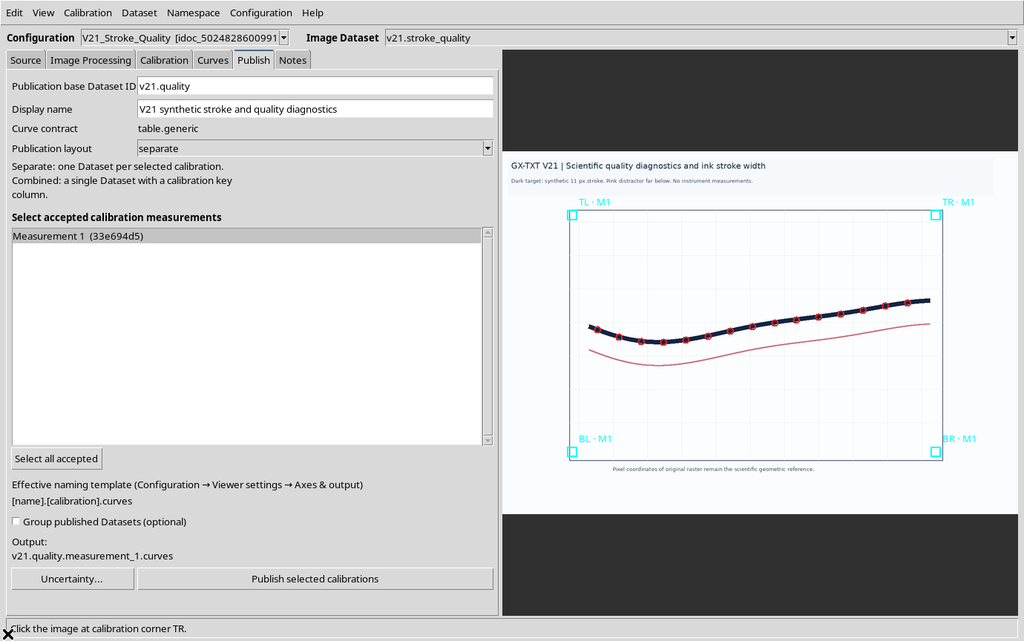
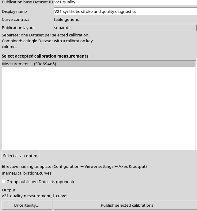
Publishing the curve is distinct from publishing a processed image. In this example the configuration contains one accepted calibration and a separate numerical Dataset is generated with the fifteen points of the first curve.
24. Quality Diagnostics Are Produced with the Dataset
At publication time, GX-TXT creates a Quality Schema v2 report associated with the numerical Dataset. It describes raster positions, distances between points, the calibration, the flags from the visual search and other structural information.
Empty curves stay included in the description of the configuration, but do not generate artificial numerical rows. This is why the publication contains fifteen rows, even though there are three curves.
25. Viewing the Dataset in the GX-TXT Browser
In the Session Dataset browser the new canonical Dataset can be selected.
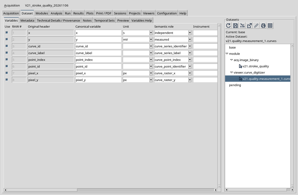
Using Open opens the CORE Scientific Dataset Viewer, which lets you view the result read-only.
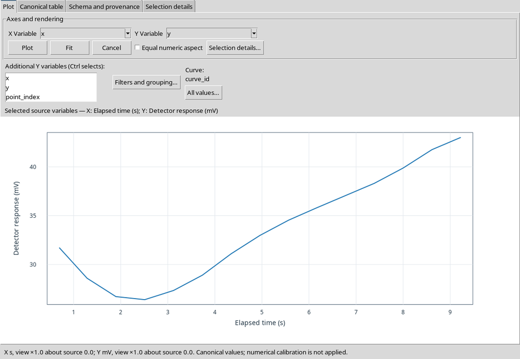
This view is distinct from the Curve Digitalizer configuration from which the Dataset was published.
26. Canonical Table: The Rows Actually Published
The Canonical table section contains the fifteen published records.
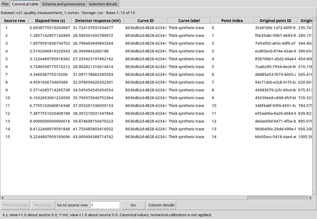
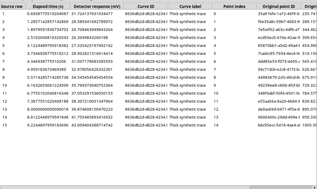
The columns include scientific X/Y, curve identifier, point order and original raster positions. The conversion between pixels and scientific units stays tied to the calibration used.
27. Reading the Quality Status Value
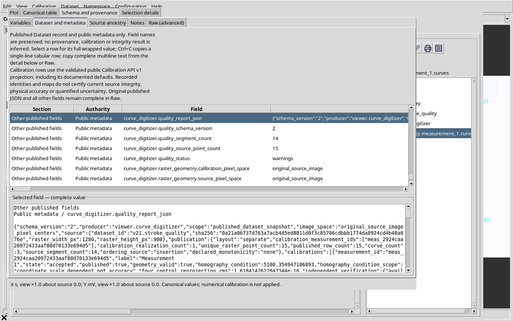
In the public metadata curve_digitizer.quality_status is available. In this example the status is warnings.
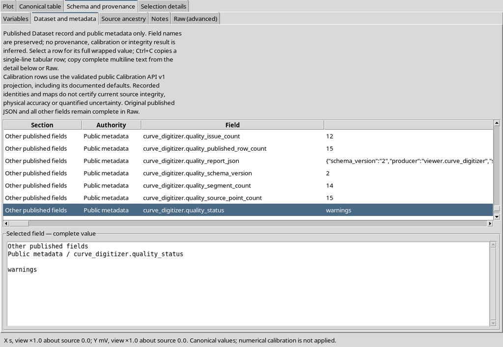
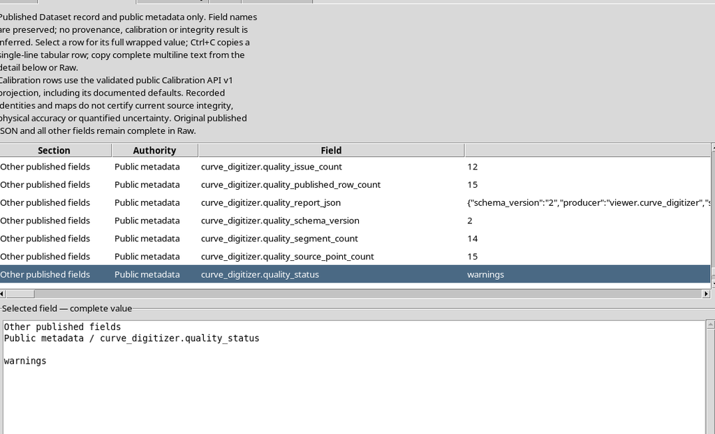
The summary value does not provide an error probability. To understand which problems were flagged, examine the full report and the curves concerned.
28. Stroke Width v1 in the Published Metadata
The Dataset also keeps a Stroke Width v1 report. The first curve is measured, with a manual median of about 10.93 px.
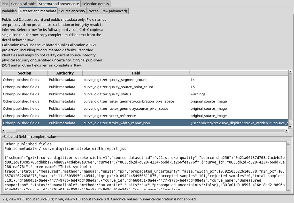
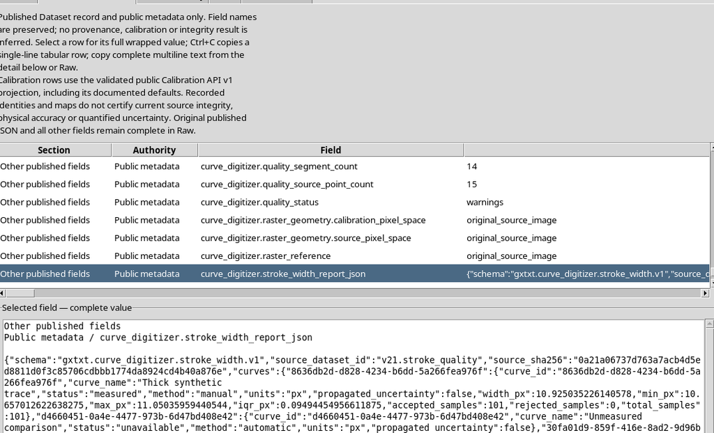
The other two are unavailable and inactive respectively. These labels make it possible to tell a measured value apart from the absence of a result.
29. What Quality Schema v2 Contains
The full report can be viewed as JSON metadata.
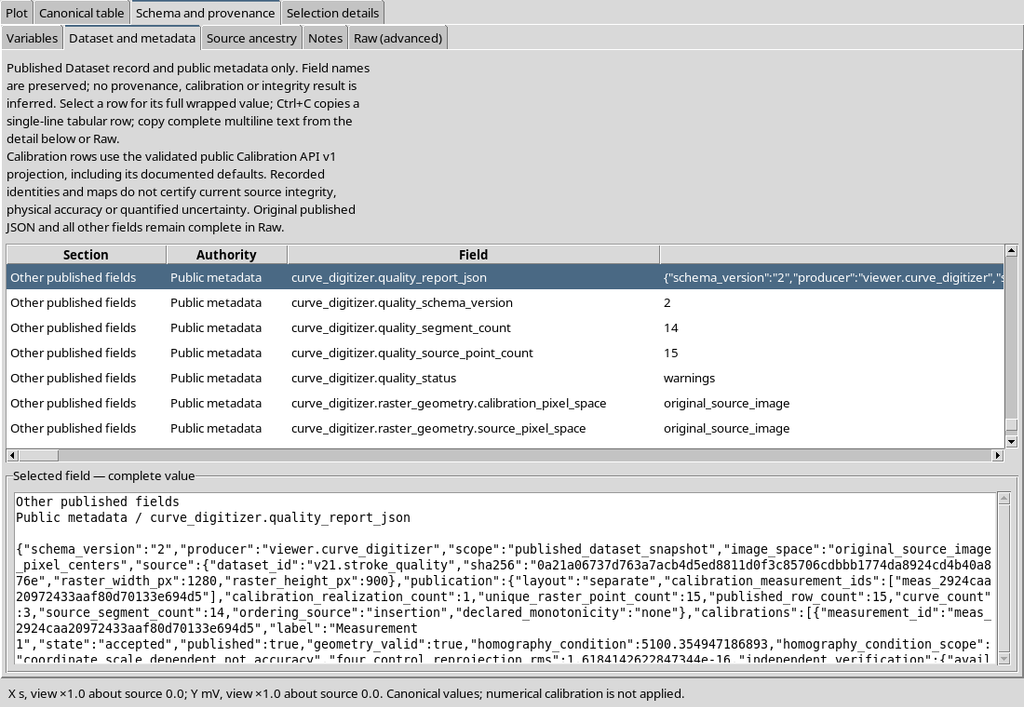
In our example there are:
| Element | Value |
|---|---|
| Unique raster points | 15 |
| Published numerical rows | 15 |
| Curves described | 3 |
| Calibration realizations | 1 |
| Segments analyzed | 14 |
| Informational flags | 10 |
| Warnings | 2 |
The report also contains the source identifier, the reference to the raster coordinates and the endpoints of the segments, so that the observations can be traced back to the original image.
30. Interpreting the Flags and Their Limits
The ten informational weak_local_contrast flags invite you to re-examine some sections of the line. The other two empty_curve warnings correspond to the curves deliberately left without points.
The contrast diagnostic uses transverse samples at about four pixels from the center of the line. In this example the dark stroke measures about eleven pixels: the side samples can still fall inside the stroke. The warning therefore does not prove that the points are wrong.
The flags are an aid to visual review, not a certified measure of accuracy.
31. Accuracy, Uncertainty and Independent Calibration
The report explicitly states that accuracy and uncertainty are not_assessed. Any independent verification of the calibration must not be invented either: if not recorded, it stays not_recorded.
A numerically small residual on the four points used to define the same calibration is not an independent accuracy validation. Estimating a metrological uncertainty requires an explicit model, with appropriate assumptions, measurements and calibration information.
The width of the stroke can be useful information in such an analysis, but it must not be turned automatically into a standard deviation.
32. Public APIs for Reading the Reports
GX-TXT numerical tools can read the diagnostics through the public APIs, without reading the private state of the Viewer.
For Quality, CURVE_DIGITIZER_QUALITY_API_v2 is available, with hasReport, read and reportJson. For the stroke, CURVE_DIGITIZER_STROKE_WIDTH_API_v1 is available, with read functions per curve, per configuration and per published Dataset.
Tcl example, in the framework environment with an active Session:
# Read published Curve Digitalizer diagnostics from public APIs.
set dataset_id "v21.quality.measurement_1.curves"

::GX::modulePublicApiActivate viewer.curve_digitizer CURVE_DIGITIZER_QUALITY_API_v2
::GX::modulePublicApiActivate viewer.curve_digitizer CURVE_DIGITIZER_STROKE_WIDTH_API_v1

if {[::GX::CurveDigitizerQuality::hasReport $dataset_id]} {
    set quality [::GX::CurveDigitizerQuality::read $dataset_id]
    set quality_json [::GX::CurveDigitizerQuality::reportJson $dataset_id]
}

if {[::GX::CurveDigitizerStrokeWidth::hasPublished $dataset_id]} {
    set width [::GX::CurveDigitizerStrokeWidth::publishedRead $dataset_id]
}
The code retrieves reports that have already been published; it does not recompute them and does not automatically produce uncertainties for the Curve Fitter or other numerical tools.
33. A Published Report Is a Snapshot of the Data
After publishing, the curve can still be edited in the Viewer. When a new scientific point is added, the previous stroke measurement of the current document is considered out of date.
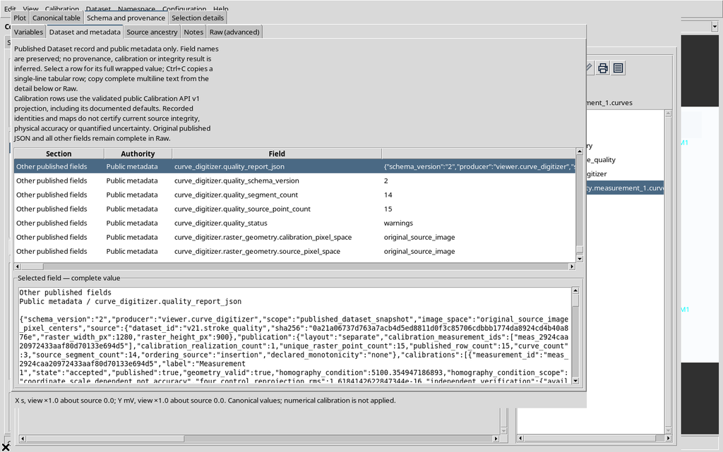
The canonical Dataset already published, however, keeps its rows and its original Quality/Stroke reports. This separation prevents published data from changing silently when the operator continues working.
34. Undo After a Later Change
Using Edit → Undo removes the point added after publication.
The configuration returns to the initial fifteen points and the previous manual thickness is shown again. The published report stays unchanged both before and after Undo.
35. Saving, Closing and Reopening
Save the configuration normally with Configuration → Save configuration. After Close and reopening in the same Session, Curve Digitalizer recovers the three curves and the manual measurement of the first one.
The published Dataset can still be viewed independently.
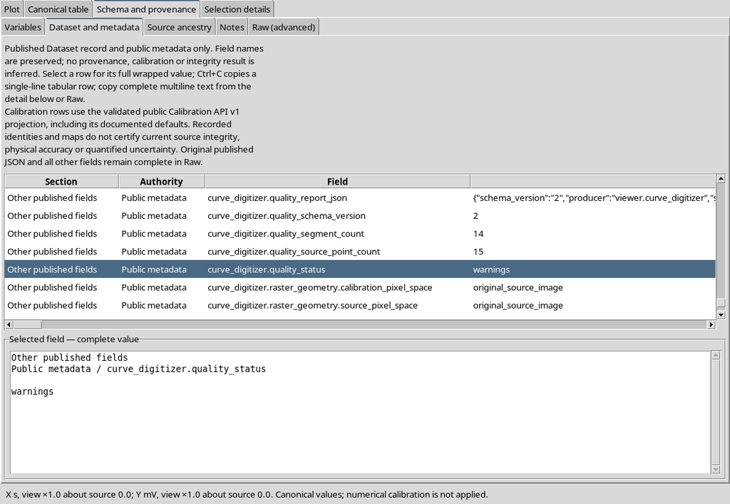
There is therefore no need to keep the same Viewer open to read the diagnostics already consolidated in the canonical metadata.
36. Recommended Operating Procedure
- Check the original image and complete an appropriate calibration.
- Acquire at least three points for automatic thickness measurement; spread more of them along the significant regions.
- Enable Measure this curve only on the series you intend to analyze.
- With Auto detect, choose a large enough Probe radius and check the accepted and rejected sections.
- If the automatic search is not reliable, use manual, Boundary A and B, then Measure two boundaries.
- Correct the boundaries with Edit boundary and Undo/Redo; do not use results that have become out of date.
- Distinguish valid, unavailable and inactive measurements in the different curves.
- Publish the numerical points explicitly, choosing the correct calibration.
- Consult the Quality v2 report and the Stroke v1 diagnostics associated with the Dataset.
- Examine the warnings on the original raster, without turning geometric statistics into unjustified uncertainties.
37. Scientific Summary
In the example, the nominal 11 px stroke was measured with an automatic median of 11.00 px and a manual one of 10.93 px. These are descriptive measurements obtained from the same image.
The published Dataset includes 15 points and a Quality v2 report with 14 segments and 12 flags to interpret. The curves that were not measured are identified without giving them artificial widths.
Stroke width, Quality diagnostics, accuracy and uncertainty are different concepts. The tools offer useful checks for the quality of the work, but the scientific validity of the digitization depends on the source, the calibration, the review of the points and any explicitly documented metrological model.