

Separate and Combined Publishing, Multiple Calibrations and Dataset Names
The GX-TXT Curve Digitalizer lets you collect several calibration realizations of the same graph. The operator can publish them in two ways: Separate, which generates one numerical Dataset for each selected calibration, or Combined, which gathers several realizations into the same Dataset, adding the calibration identity to each row.
This guide illustrates the differences in the GUI, the checks on names, the verification of coordinates in the CORE Scientific Dataset Viewer and the use of the public APIs. Two distinctions are particularly important: the active calibration is not the same as the calibration selected for Publish; moreover, twenty rows coming from ten points and two calibrations do not represent twenty independent observations.
The source used is a synthetic teaching figure. The corners of the two calibrations were intentionally chosen in slightly different positions: the numerical differences between the results serve to show the geometric propagation of the transformation, not to estimate the uncertainty of an instrument.
1. The Reference Figure
The original raster contains a dark trace and a secondary pink trace. The first is the object of the digitization.
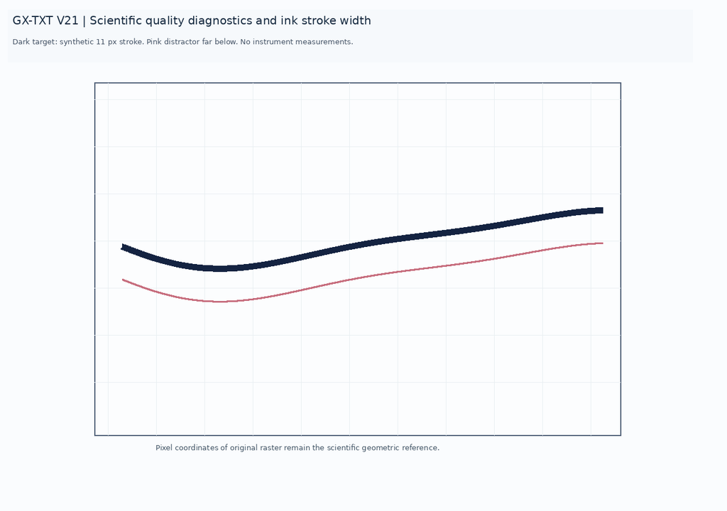
The source dimensions are 1280 × 900 pixels. The name of the source Dataset, its identity and the pixel geometry will remain unchanged throughout all the publications described.
2. A First Four-Corner Calibration
In the Calibration tab we define X from 0 to 10 s and Y from −20 to 80 mV, both linear. We select the four corners of the plot rectangle and confirm the calibration.
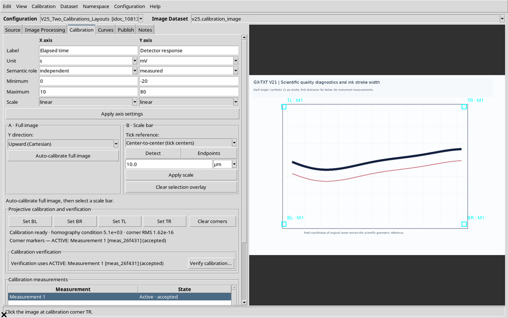
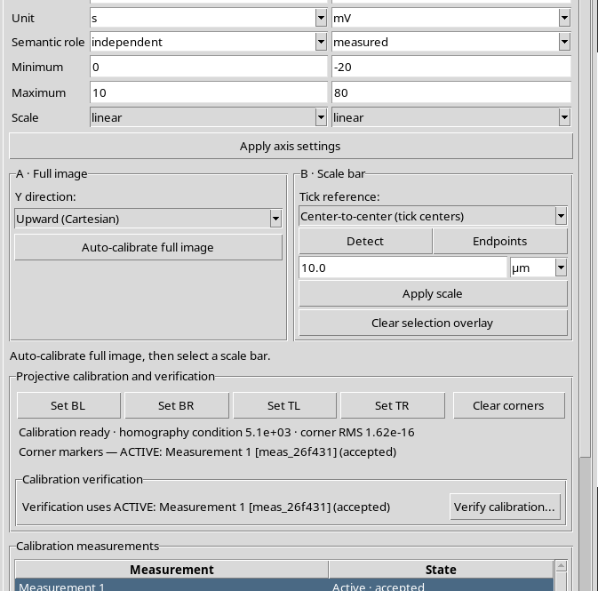
The four points define a transformation from the original pixels to the scientific coordinates. The first realization will be called Trial A.
3. Acquiring Ten Manual Points
In the Curves tab we create a scientific curve, then use Add to acquire ten points of the dark line.
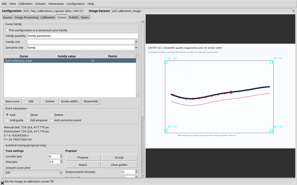
The points have an internal identifier, an original position on the raster and a calculated X/Y coordinate. Their point_id is not recreated when a different calibration is selected.
4. The Calibration Measurements Manager
The Calibration measurements section distinguishes realizations that are draft, accepted, rejected and active.
Accepted means that the realization can be used for publishing. Active, instead, indicates the transformation shown and used in the current document. The Publish tab can select an accepted calibration even when it is not the active one.
5. Creating a Second Realization
We press New in the calibration measurements manager.
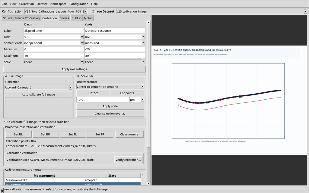
A second element is created, initially draft. The program does not treat it as already accepted: a new complete geometry must be provided and confirmed.
6. Selecting the Corners for Trial B
For the second realization we select corners slightly different from the original ones, while keeping the same image and the same physical axis limits.
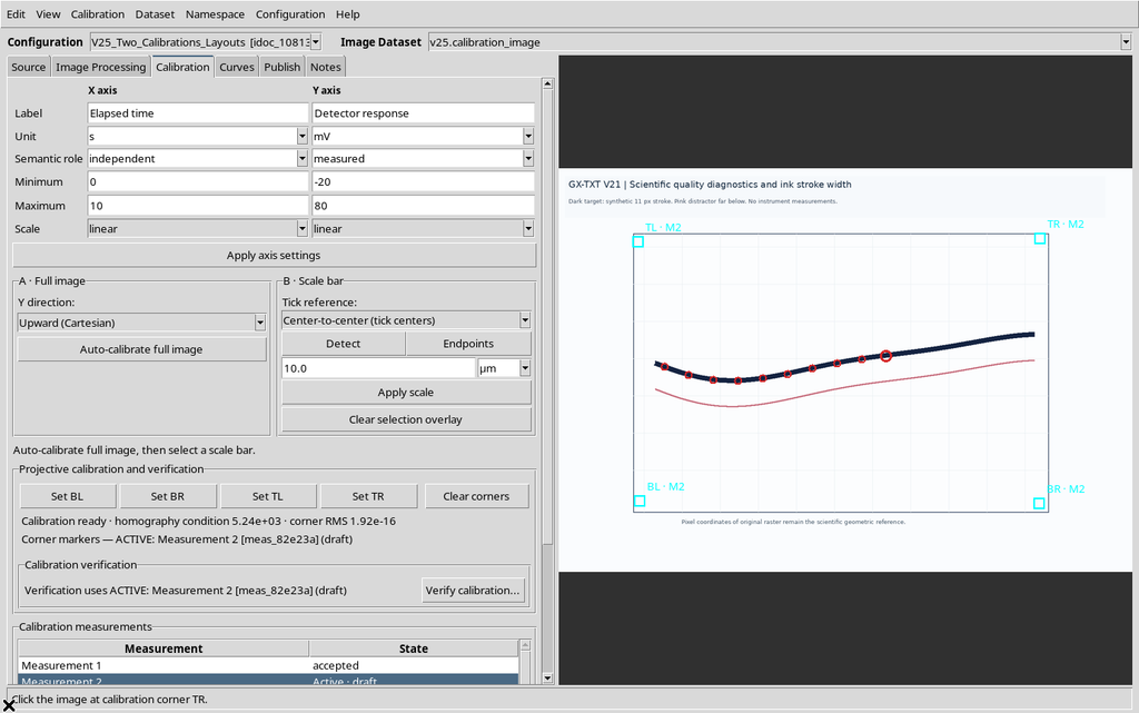
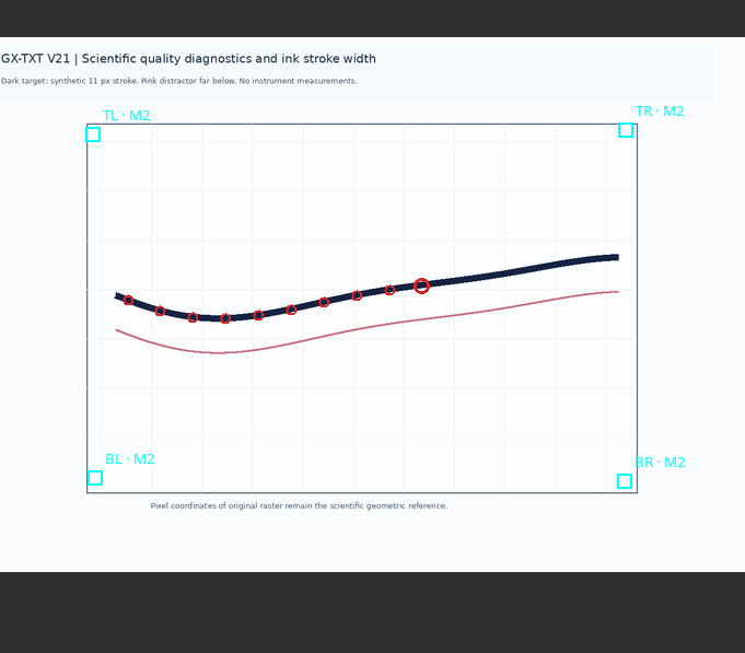
This difference is deliberately didactic. It is not an experimental replicate and does not, by itself, allow standard uncertainties or accuracy to be estimated.
7. Accepting Both Calibrations
After completing the four corners, we press Accept.
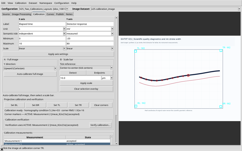
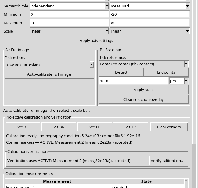
There are now two accepted realizations, with different identifiers. Both can be chosen in the Publish tab.
8. Active and Selected: What Changes?
When the first realization is activated, the X/Y coordinates of the document are recalculated on its transformation; when the second is active, they are recalculated on the transformation of the latter.
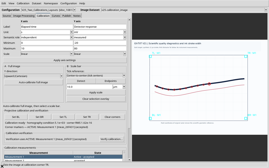
The pixel coordinates and the identifiers of the ten points remain unchanged. The Active choice does not automatically decide which calibrations will be included in a Publish operation.
9. Why the Visible Name Is Not an Identifier
To show a common mistake, we temporarily assign the same visible name to the two calibrations, while keeping their internal identifiers distinct.
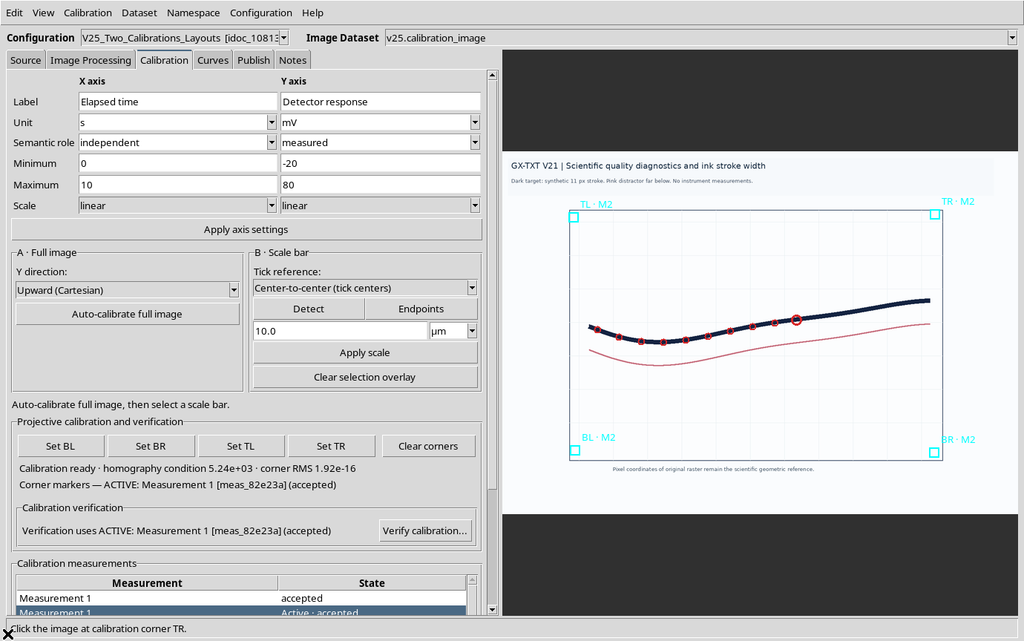
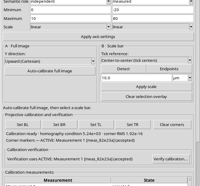
A name such as Measurement 1 is an editable description. The stable scientific identity of the realization is its measurement_id.
10. The Collision in the Publishing Plan
With the Separate layout and the default template, two calibrations with the same name generate the same planned ID.
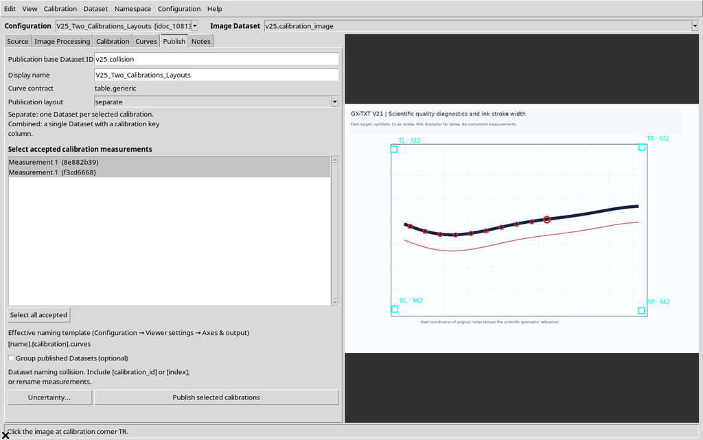
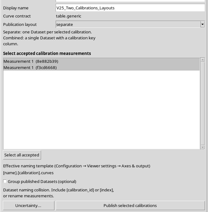
The Publish tab reports that the names collide. This happens before the canonical Datasets are created.
11. Publishing Blocked by Duplicate Names
Trying to proceed, the native message about the collision appears.
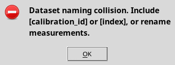
The protection prevents two Datasets with the same identifier from being produced. The problem can be solved by changing the names of the calibrations or by introducing [calibration_id] or [index] into the template.
12. Assigning Distinct Names to the Realizations
We rename the two measurements Trial A and Trial B through the Calibration measurements manager.
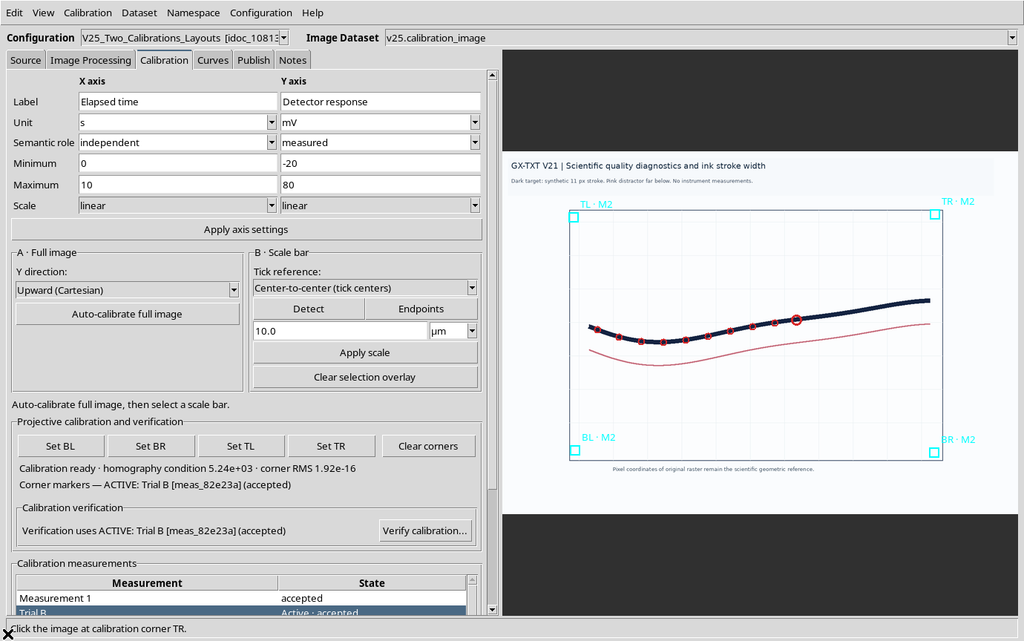
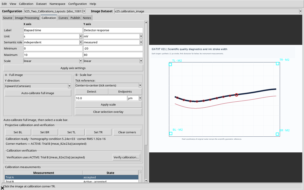
Neither the corner positions nor the original coordinates of the points have been changed: only the visible description has changed.
13. Trial B Active and Trial A Available
We activate Trial B, keeping Trial A in the Accepted state.
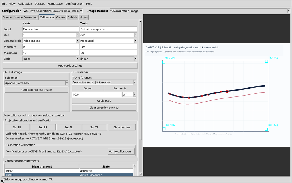
In the Publish tab we can select both realizations: publishing is not limited to the active one.
14. Separate: One Output per Calibration
We open the Publish tab, choose Separate, select both calibrations and set a base ID for the outputs.
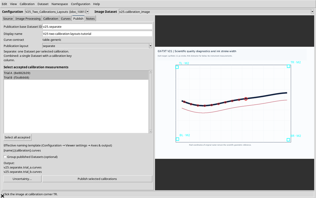
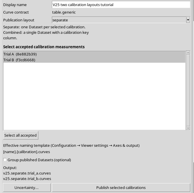
The default template [name].[calibration].curves generates two distinct names in this example: one ends in trial_a.curves, the other in trial_b.curves.
15. Publishing the Two Separate Datasets
We press Publish selected calibrations.
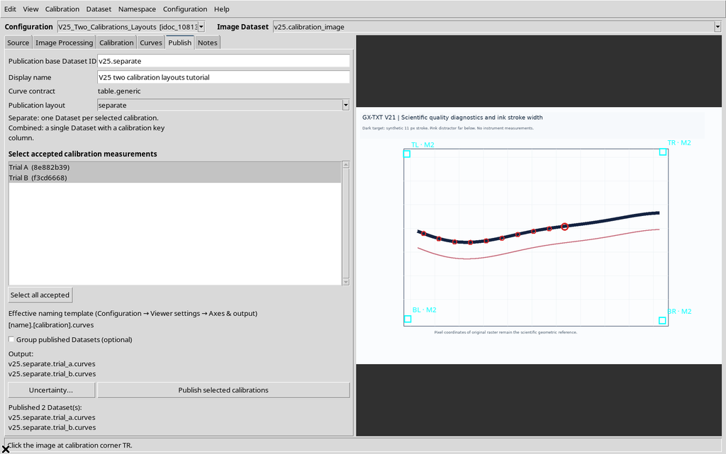
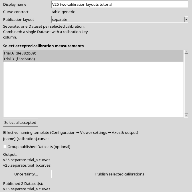
The GUI confirms two published Datasets, each with ten rows. Both are canonical GX-TXT numerical tables, separate from the original raster and from the interactive document.
16. One Origin, Two Transformations
In the two Separate outputs the ten point_id values and the pixel coordinates are the same. The scientific X/Y coordinates, instead, are slightly different, because they were calculated using two different accepted homographies.
This means that two interpretations of the same point acquisition were published. No further ten positions were acquired on the raster.
17. Combined: A Single Dataset
We go back to Publish, select Combined and keep the two accepted calibrations.
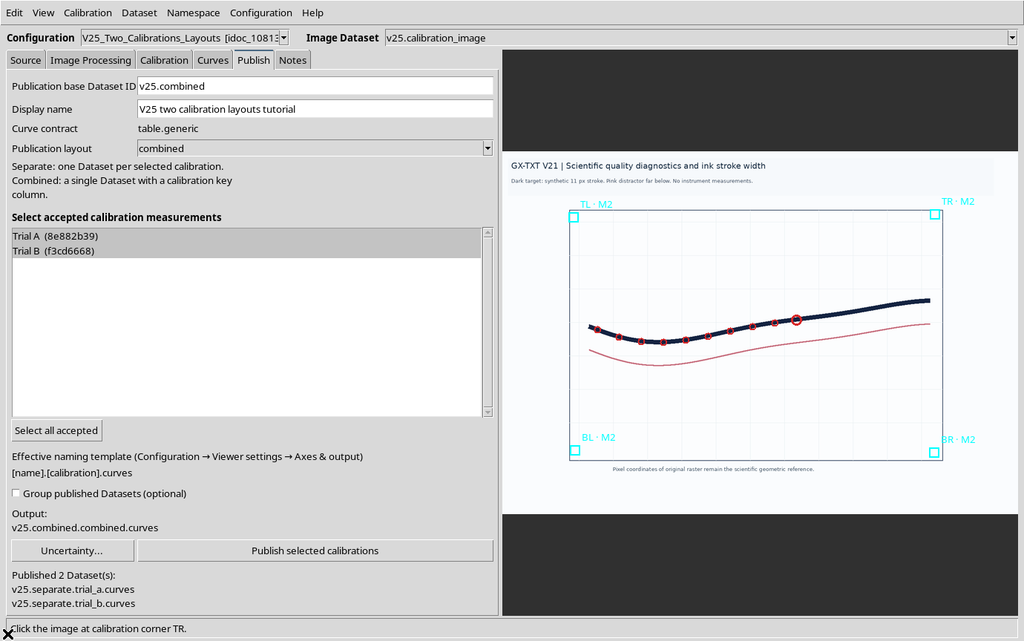
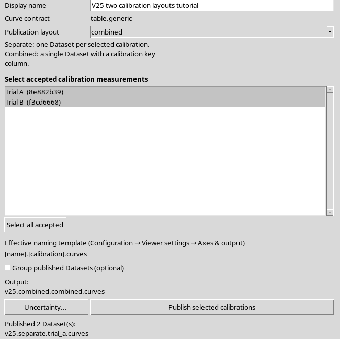
The preview shows a single ID, whose default name contains combined. This layout does not create a Dataset Group: it creates a single table with several realizations.
18. The Confirmation Warns About the Risk of Mixing Data
When Publish is pressed, GX-TXT presents a confirmation specific to Combined.
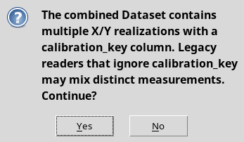
The warning is important: a program that merged all the rows while ignoring calibration_key could mix coordinates obtained with different transformations.
19. Answering No: Nothing Is Created
Choosing No, the Viewer abandons the Combined publication.
The two previous Separate Datasets remain available and no third result is created. The preview may continue to show the planned Combined ID: the preview does not prove that the Dataset has been registered.
20. Answering Yes: The Combined Result
We repeat the action and choose Yes in the confirmation.
The program registers a single Combined Dataset, made up of twenty rows.
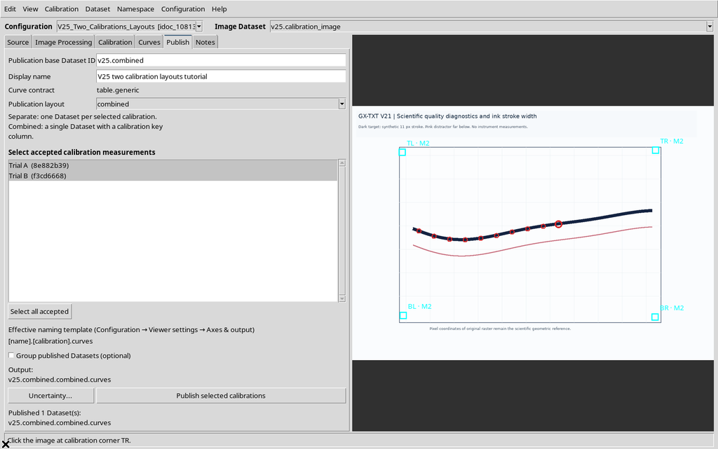
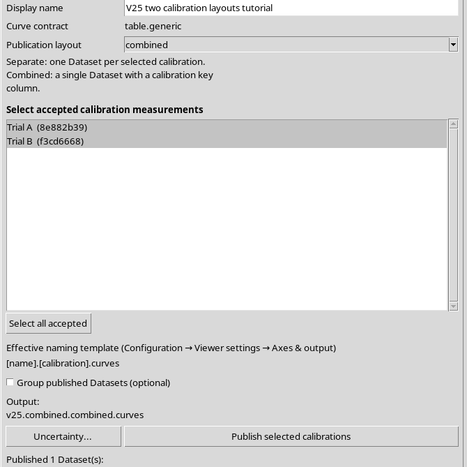
The twenty rows represent the ten original points, each expressed once with Trial A and once with Trial B.
21. Two Keys for Safe Grouping
In the Combined Dataset, grouping must not be done by curve alone. The public API declares grouping_roles = curve_key + calibration_key.
The first key indicates the series, the second the calibration realization. The descriptive fields curve_name and calibration_name must not be used as stable identifiers.
Selecting the two keys correctly prevents linking points that are physically non-homogeneous across the two transformations.
22. The Default Naming Template
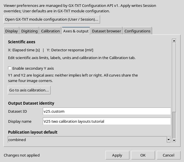
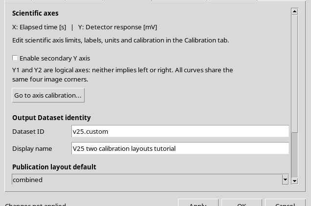
In Configuration → Viewer settings… → Axes & output the Dataset naming template box appears.
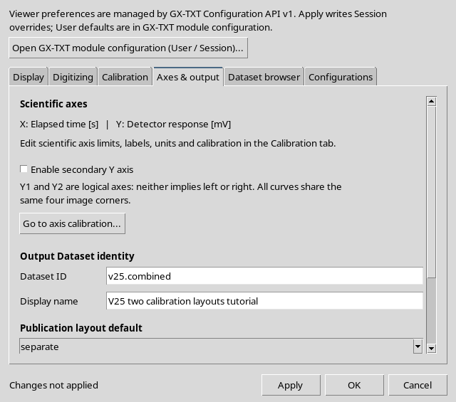
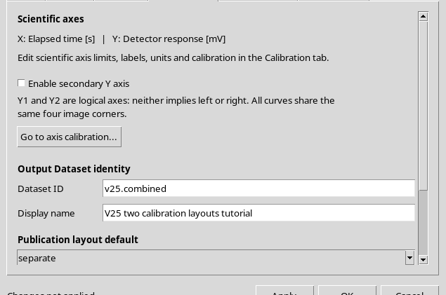
The default value is:
[name].[calibration].curves
The template is distinct from the base ID entered in Publish. The first decides how to compose the full name; the second provides the value of the [name] token.
23. The Six Recognized Tokens
The template supports these substitution elements:
| Token | Meaning |
|---|---|
| [name] | Base ID of the output |
| [calibration] | Normalized calibration label |
| [calibration_id] | Stable identifier of the realization |
| [configuration] | Normalized configuration name |
| [index] | Index of the output in the current plan, starting from 1 |
| [mode] | Separate or Combined mode |
The template must contain [name]. The permitted literal parts use ASCII characters and allowed separators; the final result must be a valid Dataset ID.
24. Unknown Tokens: Operation Rejected
We deliberately enter the non-existent token [unknown].
The editor rejects the template and indicates the recognized tokens.
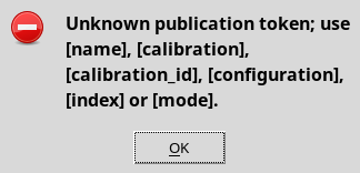
The CORE configuration is not updated by an invalid Apply attempt.
25. The [name] Token Is Mandatory
We try a second template that contains the calibration name but not the base ID.
The GUI explicitly requires [name].

This check prevents generating identifiers completely disconnected from the choice made in Publish.
26. An Unambiguous Custom Template
We choose:
[name].[index].[calibration_id].[mode].curves
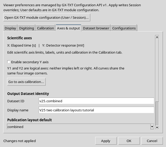
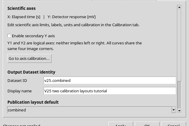
This template contains both a progressive output index and the stable calibration ID. It can avoid collisions even when two calibrations share the same label.
27. Apply Saves the Session Preferences
Pressing Apply, the GUI registers the new template.
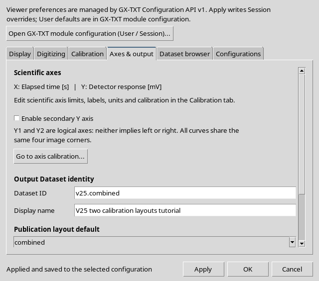
The CORE confirms that the custom template is a Session override. The default User template remains unchanged. In the example, Combined was saved as the default layout of the Session.
This does not prevent choosing Separate in the individual Publish tab, where the local choice may be different.
28. Active Calibration Versus Publish Selection
To distinguish the two concepts, we keep Trial A active in the document.
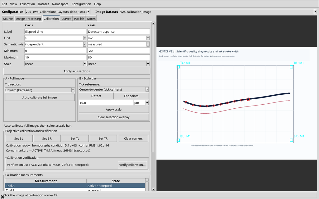
In the Publish tab it is possible to choose only Trial B. The numerical result must correspond to the selected calibration, not to the active one.
29. Preview with Two Selected Calibrations
With the custom template, we select both realizations in Separate mode.
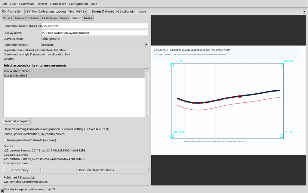
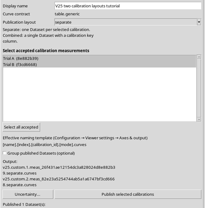
The preview produces two names: the first uses index = 1, the second index = 2. Both include their respective calibration_id.
30. Selecting Only Trial B
Now we choose only Trial B, leaving Trial A active.
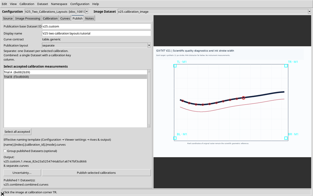
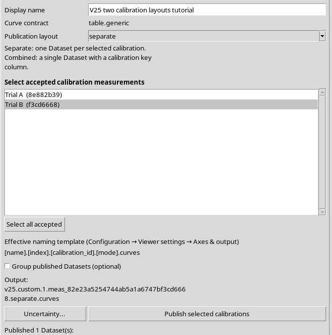
Since the plan contains a single output, the index restarts from 1. It is not the immutable index of the calibration in the measurements manager, but the position of the output in the current publishing plan.
31. Actually Publishing the Custom Name
We confirm Publish.
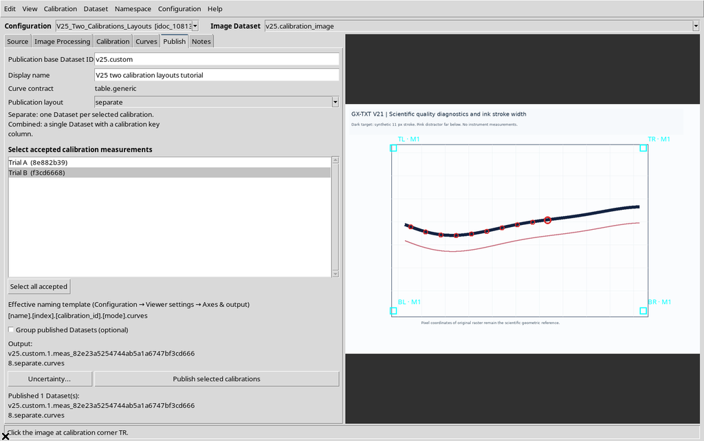
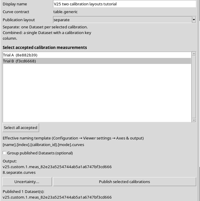
The resulting Dataset contains ten rows of Trial B, with the same transformation as the previous Separate publication of Trial B. The custom ID is longer, but it does not change the coordinates.
32. The Template in Combined Mode
If we choose Combined again with both calibrations, the template preview becomes a single ID containing the values index = 1, calibration_id = combined and mode = combined.
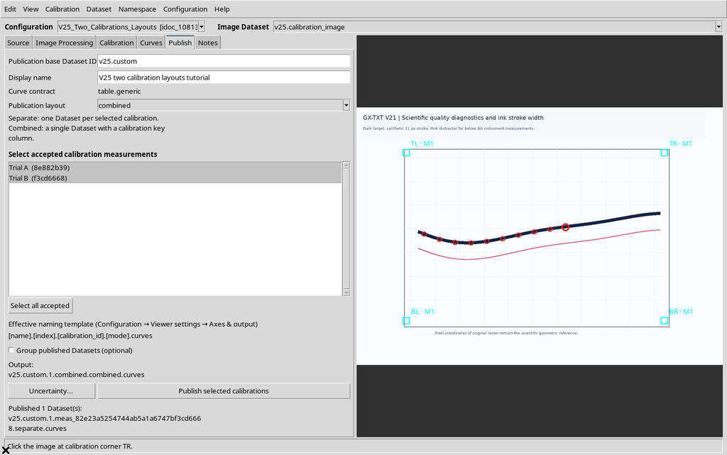
It is a new preview, not a further publication. The choice of tokens depends on the actual layout selected, not only on the Session default.
33. Viewing Trial A in the CORE
We open the Separate result of Trial A from the GX-TXT Dataset browser.
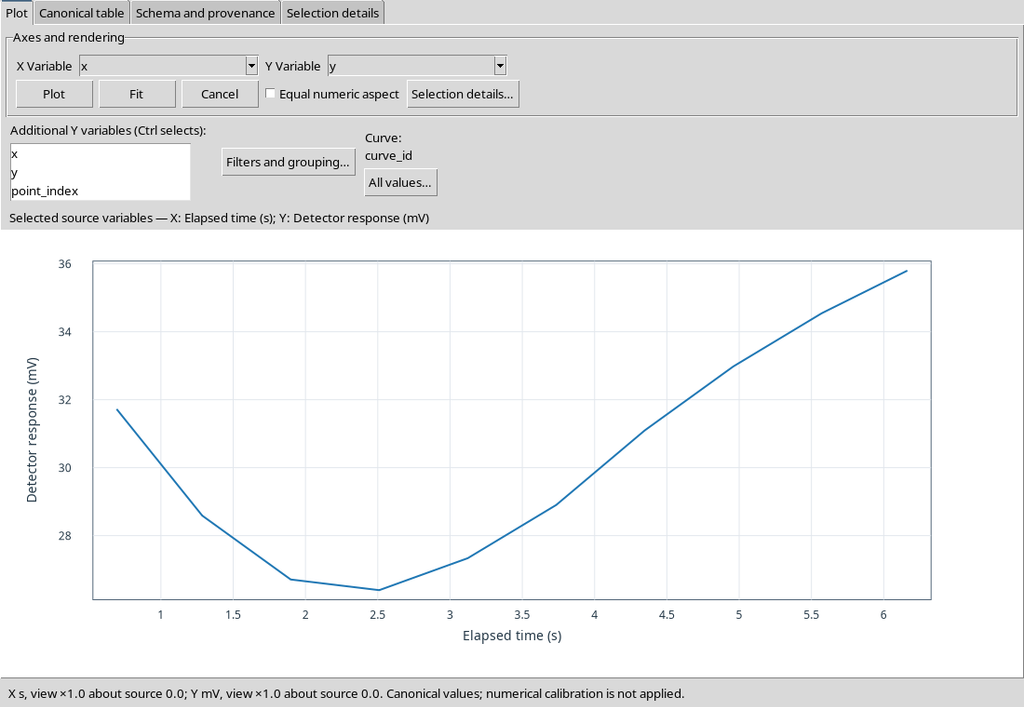
The CORE Scientific Dataset Viewer displays the curve in the Plot view. The canonical table is the reference for checking the published coordinates exactly.
34. The Ten Rows of Trial A
In the Canonical table tab we find ten rows.
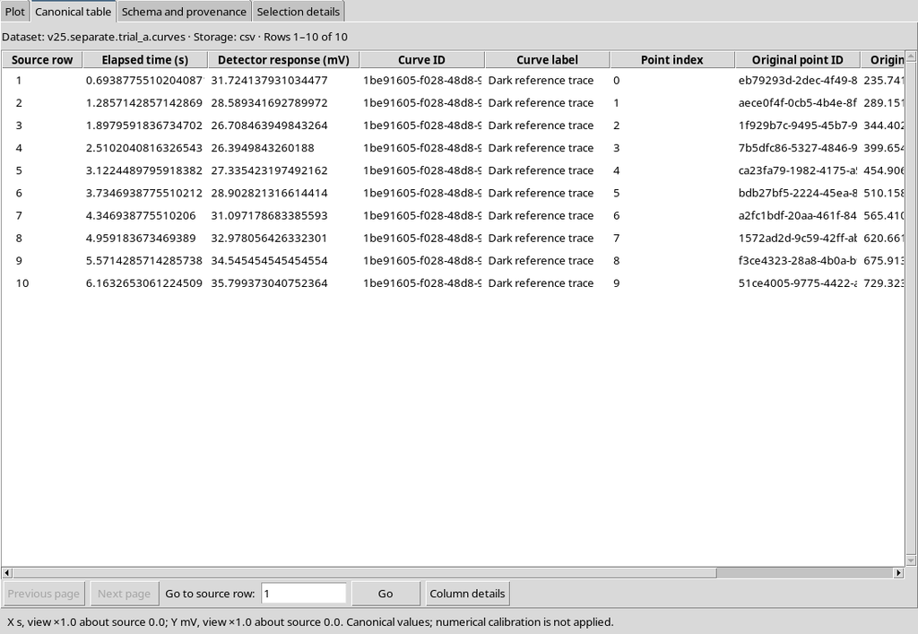
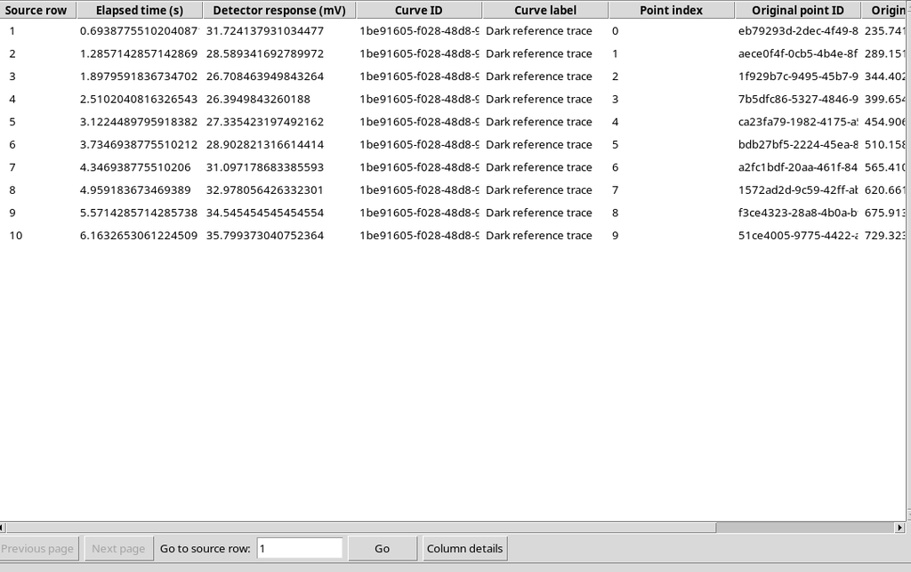
The Variable Schema v3 describes the eight variables of the Separate Dataset: scientific coordinates, curve and point identifiers, order and raster positions.
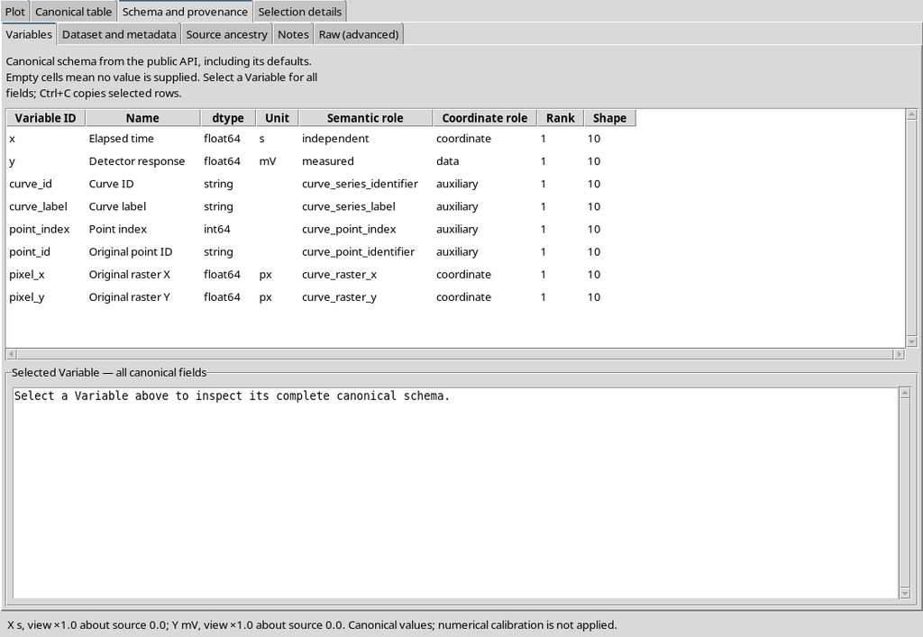
For a Separate Dataset the calibration ID is kept in the Dataset metadata, not repeated as a field of each individual row.
35. Opening Trial B as a Standalone Dataset
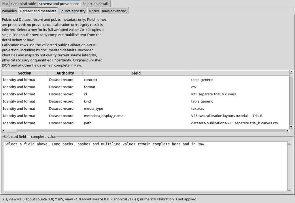
We open the second Separate Dataset in the CORE Viewer.
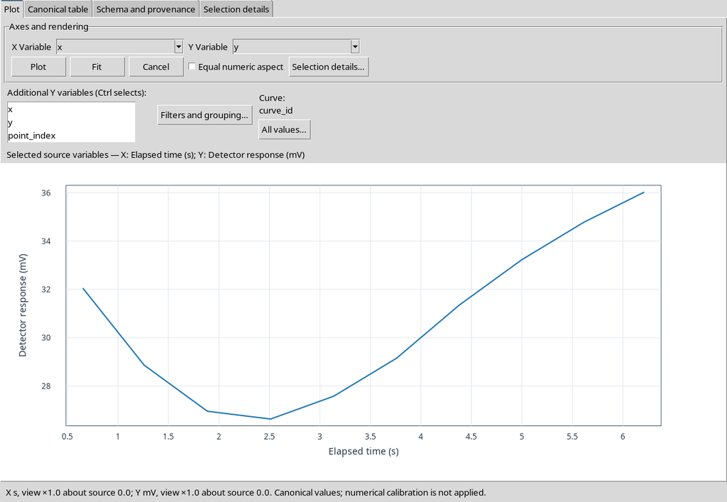
In this case too, the result is a standalone canonical object, with ten rows and a reference to its own calibration realization.
36. The Trial B Coordinates Are Different
The canonical table of Trial B contains the same ten identifiers and pixels as Trial A.
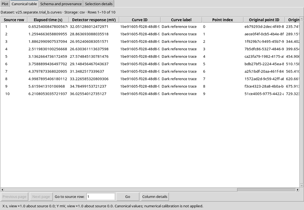
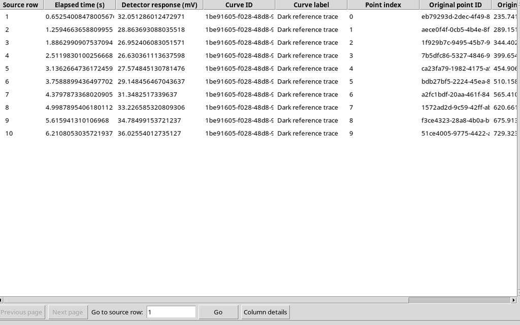
The X/Y values differ: in the example, the maximum deviation observed for the same ten points is about 0.0475 s on X and 0.3272 mV on Y. It is an effect of the two synthetic calibrations, not an estimate of instrumental accuracy.
37. Selecting the Combined Result in the Browser
In the GX-TXT catalogue we can choose the Combined Dataset, distinct from Trial A and Trial B.
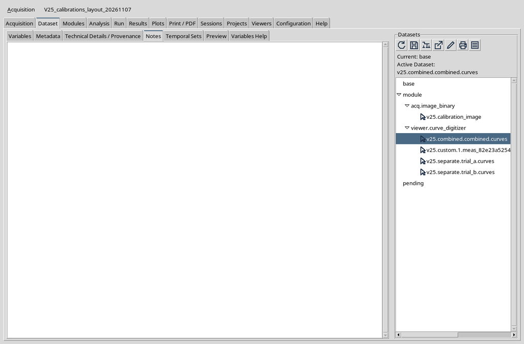
Its identifier and its canonical payload are different from the two Separate publications.
38. The Plot View Does Not Resolve the Semantics on Its Own
The CORE Scientific Dataset Viewer also opens the Combined.
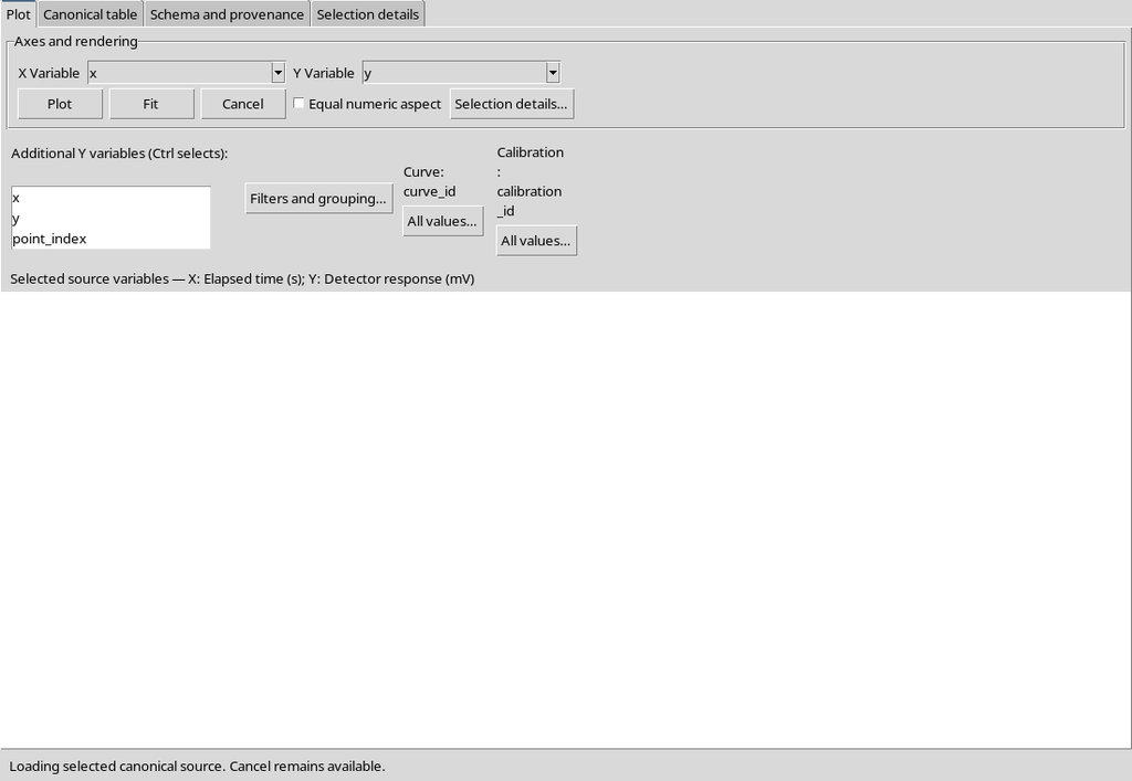
A graphical representation that ignores the two realizations may be misleading. The calibration key is an integral part of the meaning of the records.
39. The Combined Table Has Twenty Rows
The Canonical table section shows twenty records, with the additional fields calibration_id and calibration_label.
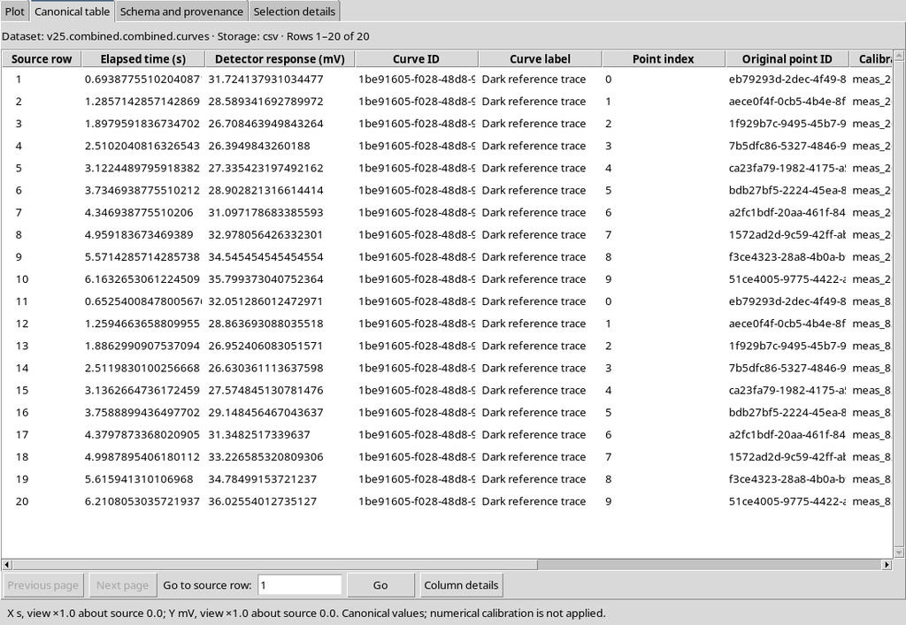
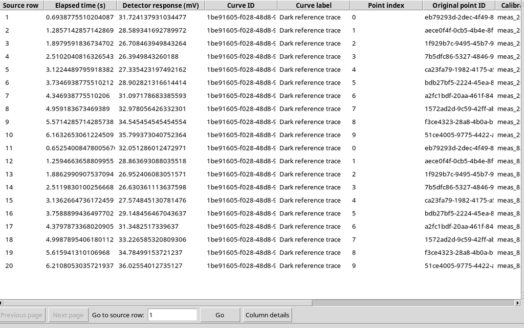
The first ten rows are associated with Trial A and the following ten with Trial B. The same point_id values can therefore appear twice, but each row is also distinguished by its calibration_key.
40. Ten Variables in the Variable Schema v3
The Combined declares ten variables, compared with the eight of the Separate.
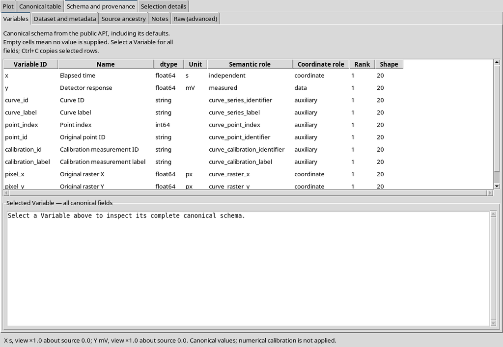
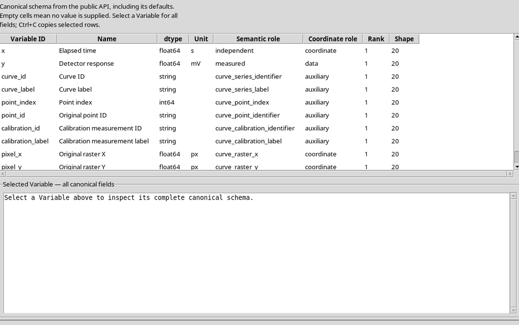
The additional semantic roles are calibration_key and calibration_name. The second is a description, the first is the stable identifier. The CORE declares that the full grouping uses curve_key and calibration_key.
41. Provenance and Transformations
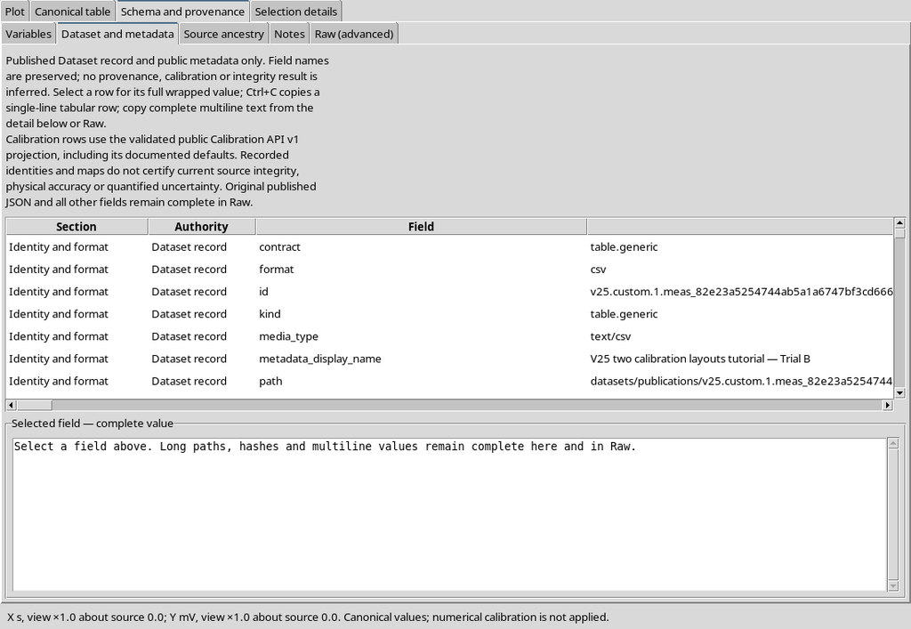
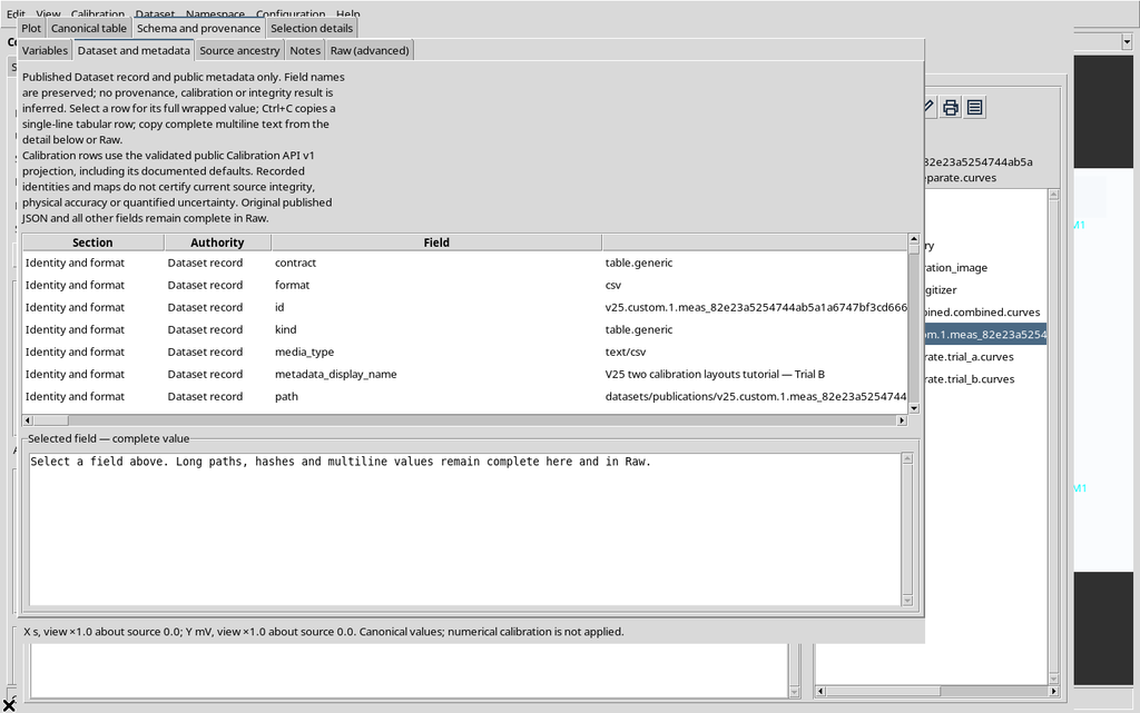
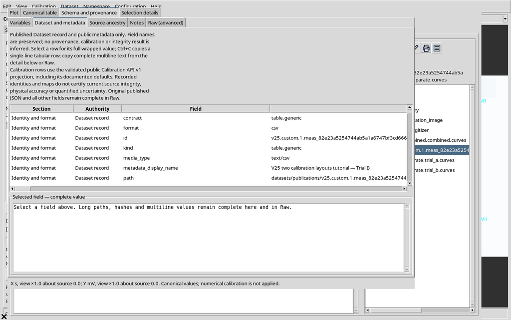
The metadata of the Combined preserve the origin and the published calibration realizations.
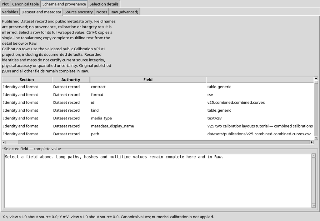
The Source ancestry section shows the link with the original image.
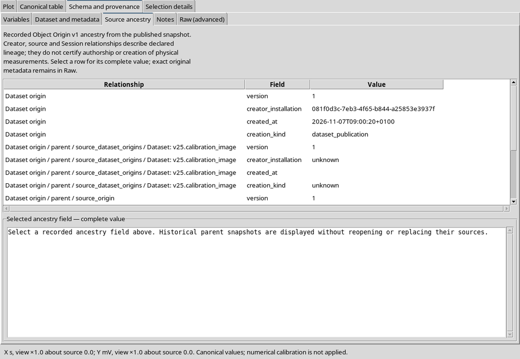
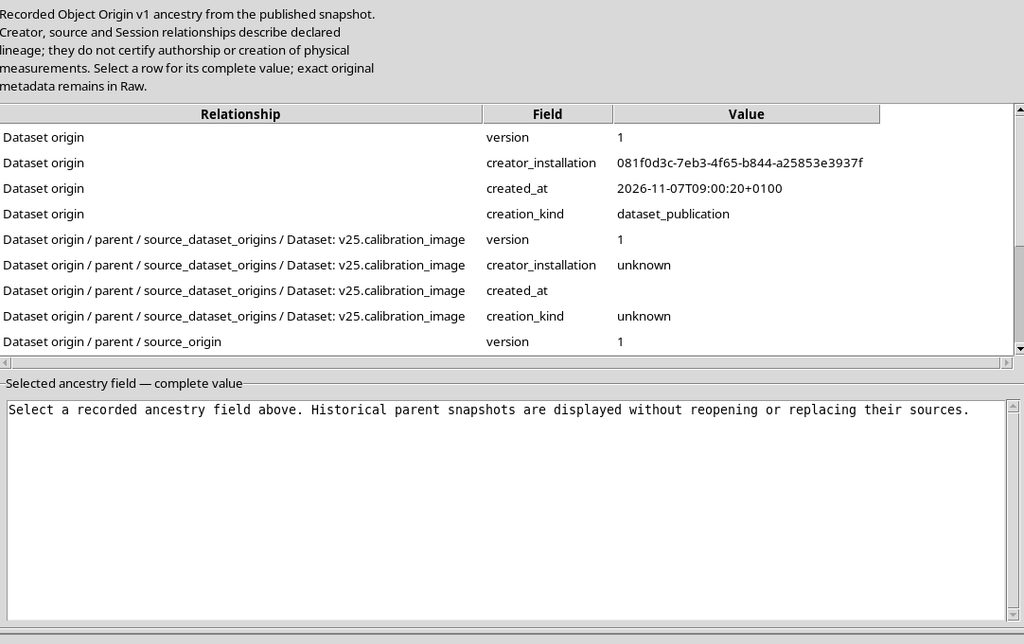
This link makes it possible to trace the coordinates back to the raster and to the appropriate transformation, avoiding confusion between two interpretations of the same pixel position.
42. Verifying the Dataset with a Custom Name
The custom publication of Trial B alone is also available in the Dataset browser.
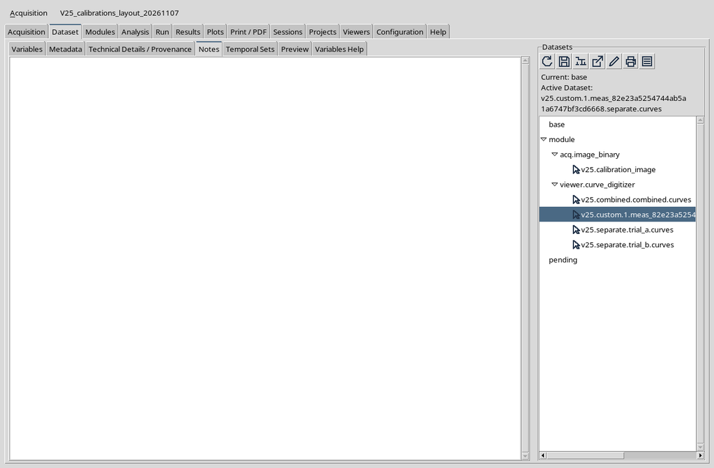
The CORE Scientific Dataset Viewer shows its Plot and Canonical table.
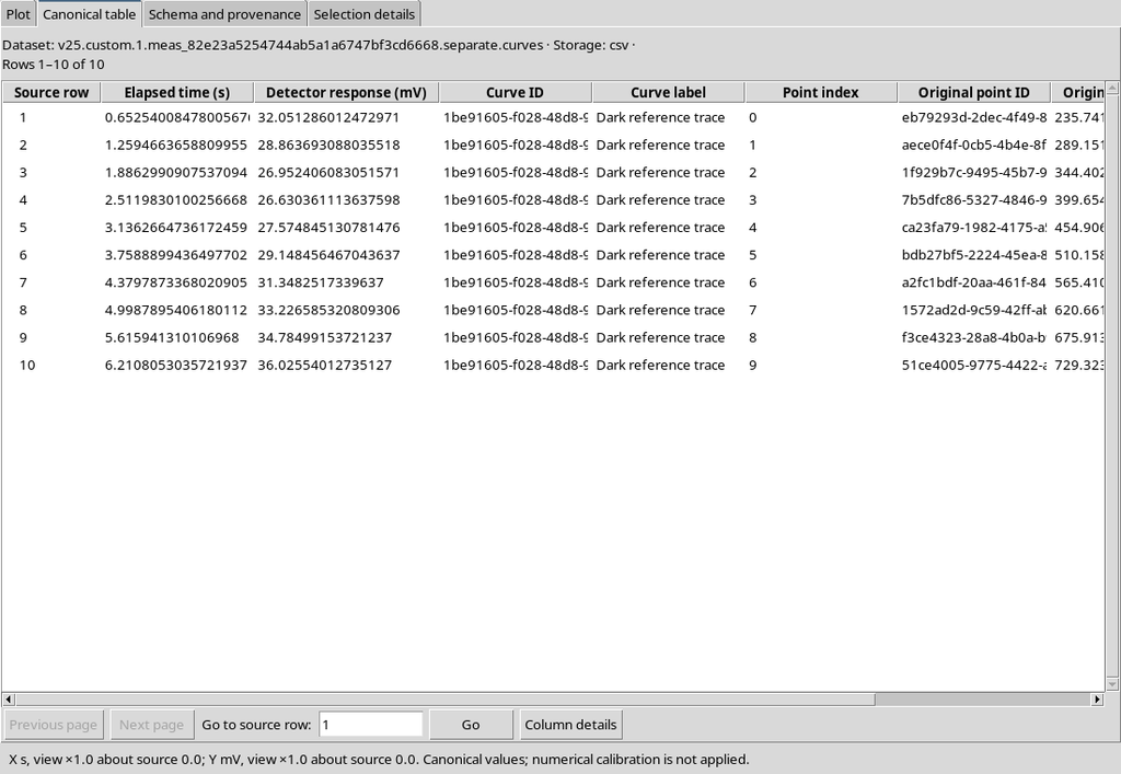
The metadata confirm that the Trial B realization was published, even though Trial A was active during the procedure.
43. Saving the Work and Checking the Reopening
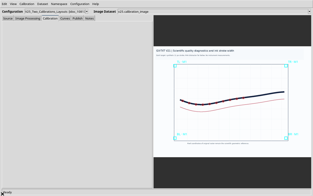
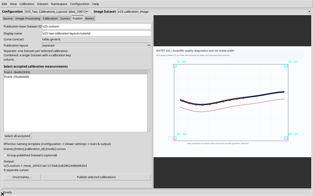
Before closing the Viewer, the Calibration manager shows both accepted realizations.
The Publish tab still contains the local Separate choice, even though the default layout of the Session is Combined.
After Configuration → Save configuration, Close and Reopen, the ten points and the two calibrations are still available.
The Publish tab still allows choosing the outputs and the custom template.
44. Session Preferences and Source After Reopen
Opening Viewer settings, the custom template and the default Combined layout are found again.
The original source and the four numerical Datasets already published are still available.
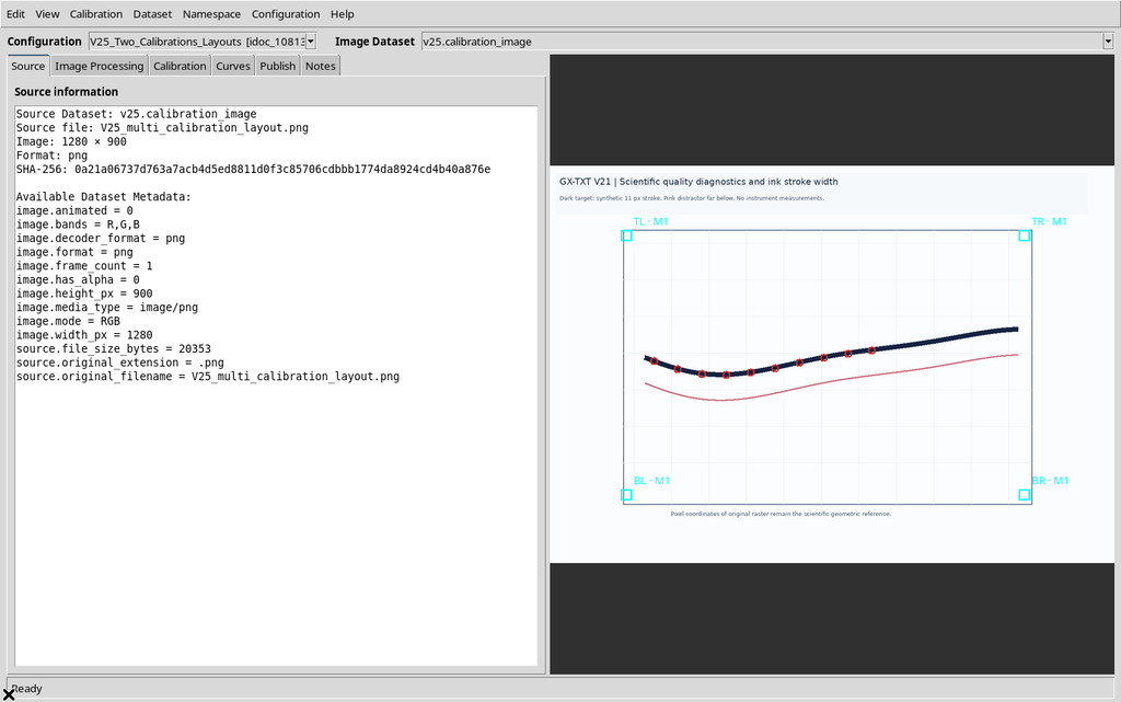
The identity of the canonical outputs is independent of whether the Viewer is open; tables already published are not rewritten by reopening.
45. Checking the Selection After Reopen: An Important Precaution
After reopening the Viewer, Publish may restore a selection different from the one saved. In the example only Trial B had been selected, while Trial A was active.
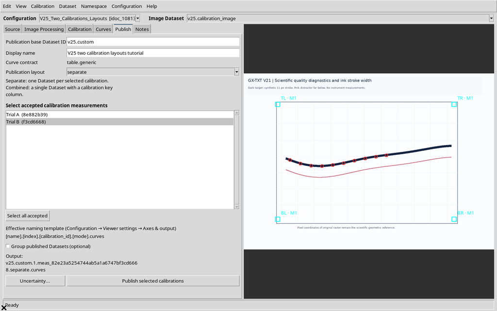
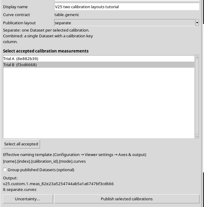
After reopening, the GUI showed Trial A selected instead of the previously chosen Trial B.
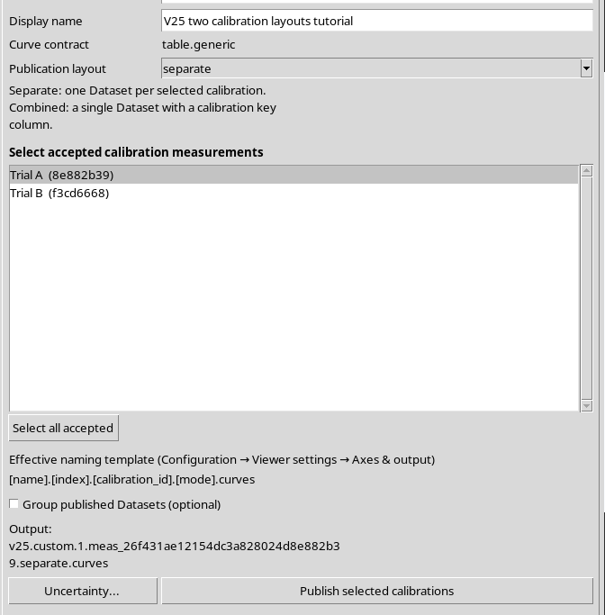
After each reopening, check and, if necessary, reselect the calibrations in Publish before publishing. The previous canonical outputs are not modified: the problem concerns only the selection restored in the Interactive Document, not the transformations already published.
46. Public APIs: Recognizing the Layout
A program that works on the Datasets should resolve the columns and their roles through the public APIs, without relying on the position of the CSV columns.
In the framework, with the relevant Session active, use the actual identifiers of the Dataset and of the calibration realization in place of the example values in the code:
# Activate versioned, public Curve Digitalizer Dataset Schema API.
::GX::modulePublicApiActivate viewer.curve_digitizer CURVE_DIGITIZER_DATASET_SCHEMA_API_v1

set dataset_id "example.combined.curves"
set manifest [::GX::CurveDigitizerDataset::read $dataset_id]

# The full set of grouping roles may contain more than one key.
set roles [dict get $manifest grouping_roles]
set curve_column [dict get $manifest columns curve_key]

if {[dict exists $manifest columns calibration_key]} {
    set calibration_column [dict get $manifest columns calibration_key]
}

# Read a bounded canonical subset for one calibration realization.
set measurement_id "example_measurement_id"
set rows [::GX::CurveDigitizerDataset::rasterPoints
    $dataset_id "" 0 100 $measurement_id]
The rasterPoints signature accepts a filter on the calibrationKey parameter, in addition to the optional curveKey filter. The number of rows returned must be checked; you must not assume that it corresponds to the entire Combined Dataset.
47. Calibration API: Reading Each Realization
The CURVE_DIGITIZER_CALIBRATION_API_v1 API lets you consult the published realizations and apply the appropriate transformation to the original pixels. In the following Tcl block, dataset_id is the same identifier set in the previous example.
# Activate the public calibration manifest API.
::GX::modulePublicApiActivate viewer.curve_digitizer CURVE_DIGITIZER_CALIBRATION_API_v1

set calibrations [::GX::CurveDigitizerCalibration::replicates $dataset_id]

foreach cal $calibrations {
    if {![dict get $cal valid]} {
        continue
    }

    set mid [dict get $cal measurement_id]
    set original_pixels {{235.74 441.71}}

    set xy [::GX::CurveDigitizerCalibration::transformPoints
        $dataset_id $original_pixels pixel_to_scientific $mid]
}
The realization must be indicated through measurement_id, not deduced from its label. The same API allows the inverse scientific_to_pixel transformation with the specified calibration.
48. Rules for Choosing Separate or Combined
Use Separate when it is useful to treat each calibration as a distinct Dataset, with its own identity and its own table. Handling is simpler for consumers that are not designed to distinguish several realizations in the same output.
Use Combined when a single table with several realizations is needed, but only if the downstream tools respect calibration_key and the CORE confirms that the physical units of the axes are compatible.
Combined publishing in fact requires the same physical X units for all the selected calibrations and the same Y units. It is not a way to directly merge incompatible quantities.
49. Limits of the Procedure
This guide examined one curve, two accepted calibrations and four test publications, all coming from the same synthetic raster.
We did not create new independent measurements, calculate confidence intervals or declare metrological uncertainties. An uncertainty model reviewed for one calibration must not be automatically transferred to another. Combined publishing of several calibrations with reviewed numerical uncertainty is not scientifically supported by this version: use Separate or disable the declaration, when appropriate.
Dataset Groups, dual Y axes and multi-Y schemas are covered in a later guide; they are not implied by the simple Combined layout.
50. Recommended Operating Procedure
- Keep the original raster and acquire the scientific points from an identified source.
- Create and accept the calibration realizations, keeping their measurement_id values distinct.
- Assign descriptive names, but do not use the label as a stable scientific identity.
- Check the difference between the active measurement in the Viewer and the measurements selected in Publish.
- Choose Separate for distinct Datasets or Combined for a single table with calibration_key.
- Check the ID preview before publishing. Use [calibration_id] or [index] when labels can collide.
- For a custom template, include [name] and only authorized tokens.
- In Combined, read the warning and proceed only if the downstream tools understand the calibration keys.
- Check the Datasets in the CORE, comparing the records with the realizations through the public APIs.
- After Save/Close/Reopen, check the selected calibrations in Publish again before confirming a further output.
Conclusion: Separate and Combined allow two different organizations of data obtained from the same pixel points. Scientific correctness depends on maintaining calibration identities, unambiguous naming and reading the semantic roles, not only on the number of rows in the table.