

Dataset Preview — Viewing Published Curves
The Curves tab of the Dataset Preview lets you consult the scientific points published by the Curve Digitalizer. Unlike the preview of an image, it presents a series of numerical curves with physical axes, using the native Plot Dataset API v4 engine. In this guide we prepare three practice curves and open them in the framework’s integrated Preview.
The example uses a synthetic graph with five coloured traces. We digitize three of them, with eight points each, obtaining 24 canonical scientific rows. These are not experimental measurements: the case serves to distinguish the source image, the calibrated coordinates, the publication and the subsequent consultation in the Dataset Preview.
1. From the Curve Digitalizer to the Dataset Preview
The Curve Digitalizer Viewer lets you choose pixels on the raster and convert them into scientific coordinates through a calibration. The Dataset Preview, instead, reads the results after their publication in the CORE. It is important to distinguish the two phases: the presence of a curve drawn on the Viewer screen does not guarantee that a consultable numerical Dataset already exists.
To practise with Curves, start from a Session with a compatible image, a scientific configuration, at least one accepted calibration and points belonging to defined curves.
2. The Calibration Defines the Axes of the Future Plot
Before publishing, the Viewer’s Calibration tab defines the X axis and the Y axis. In the example the quantities are Elapsed time (s) and Detector response (mV), with linear X from 0 to 10 s and linear Y from −20 to 80 mV. Four references BL, BR, TL, TR allow the geometric transformation to be calculated.
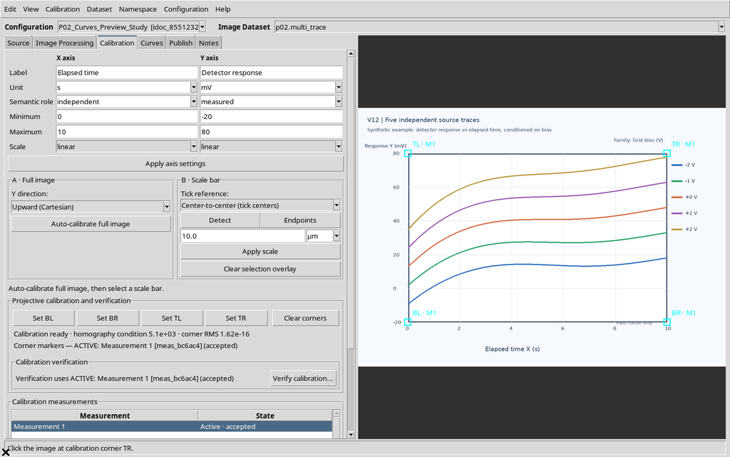
Check for the accepted label before moving on to the curves. The display scale of the image and the numerical limits of the axes are different concepts.
3. The First Curve and Its Points
In the Curves tab, the New curve command creates an independent series. Give it a descriptive name and use Add mode to insert the points along the first trace of the raster. In this exercise the first curve is called Bias -2 V.
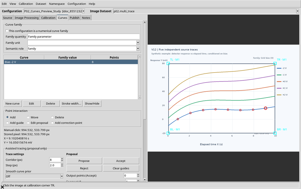
The Viewer stores the point in the image and the corresponding scientific position; there is no need to draw a new plot manually to publish it.
4. Adding a Second Curve
Repeat New curve for a second series, for example Bias -1 V. During insertion always check which curve is active: a click on the raster assigns the new point to the selected series.
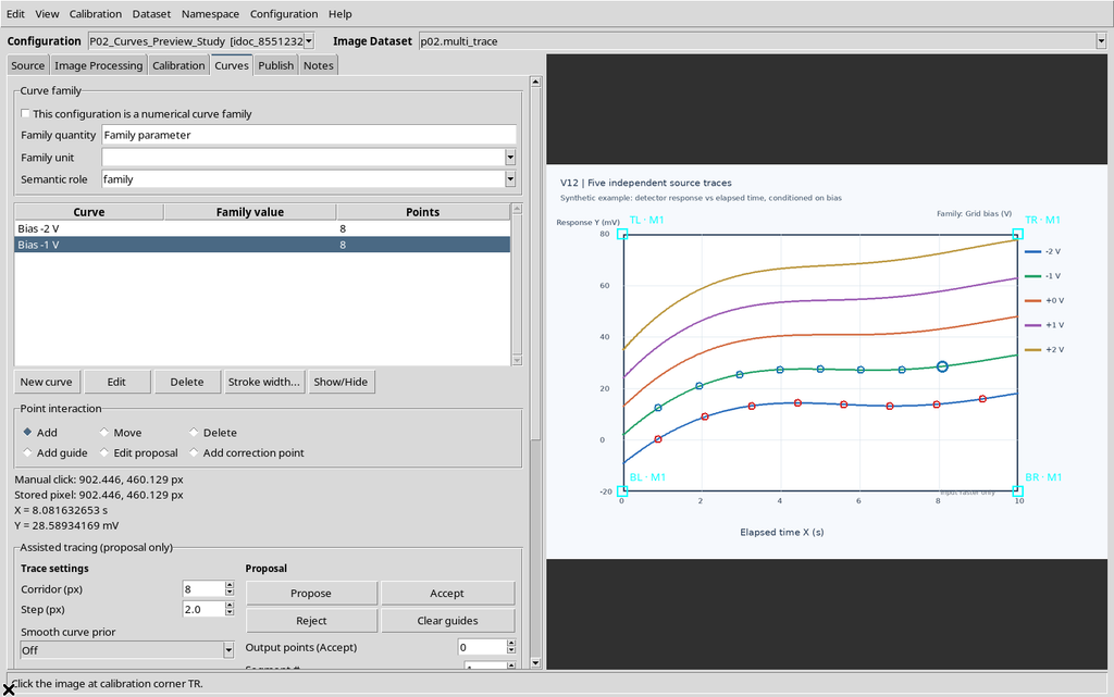
Here the two curves share the same calibration and the same X/Y units, but they keep independent numerical identities and point sequences.
5. Adding the Third Curve
Create Bias +0 V, again with eight points. For a linear demonstration it is enough to use some representative positions of the trace, provided the order and the association with the correct curve are maintained.
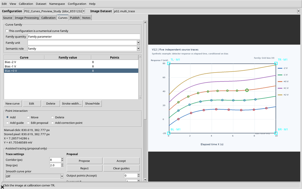
The other two traces of the source figure simply remain in the raster: they do not become numerical curves just because they are drawn.
6. Checking the Three Series Before Publish
Review the Curves table, the number of points for each series and the active calibration. The example contains three independent series, each with eight points, for a total of 24.
Any points moved or deleted in the Viewer affect the data to be published; a later change of visibility in the Preview, instead, must not modify the registered Dataset.
The screenshot with the third curve already completed shows the presence of the three series: before publishing it is enough to check the point counters in Curves, the active curve and the accepted calibration. The eight coordinates of each series remain distinct; the traces still visible on the raster must not be interpreted as further numerical curves.
7. Preparing the Numerical Dataset
Open the Viewer’s Publish tab. Check the accepted calibration, the publishing mode, the proposed identifier and the readable name of the Dataset. For the example the separate mode was used, with a single accepted realization.
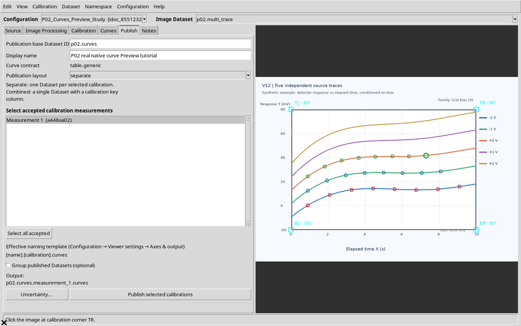
The ID identifies a canonical object of the Session. It is not the name of the original image and must not be interpreted as the number of the curve.
8. Running Publish and Checking the Result
Press Publish selected calibrations. A successful publication registers the new scientific Dataset in the CORE, distinct from the Viewer’s interactive document.
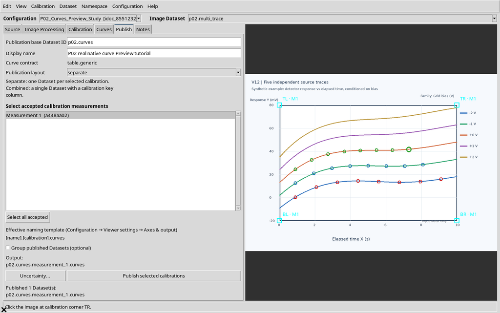
Before continuing, make sure the Dataset is visible in the framework browser. The success message alone, without checking the Session and the output, does not replace verification of the data.
9. Opening the Published Dataset in the Framework
Go back to the main GX-TXT window and choose Dataset → Preview. From the Datasets panel, locate the numerical Dataset just produced, not the previous Image Dataset. In the example the result is a table.generic object with 24 rows.
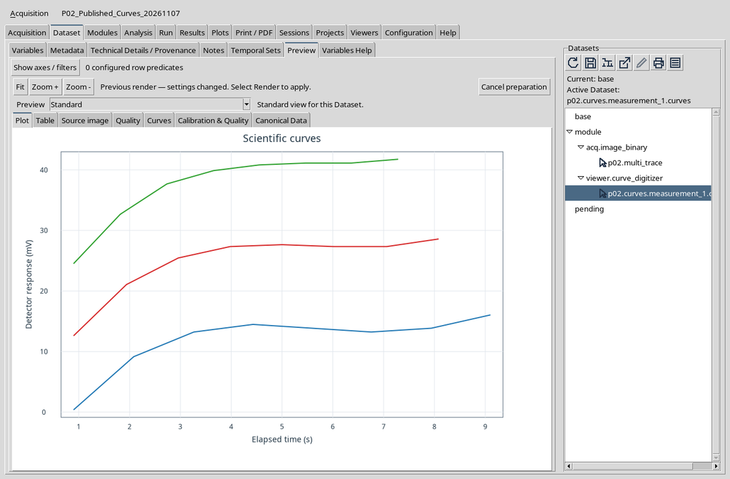
The Preview recognizes the link with the Curve Digitalizer and offers further specialized tabs.
10. The Preview Has Several Views of the Same Dataset
The central pane may show Plot, Table, Source image, Quality, Curves, Calibration & Quality and Canonical Data, in addition to the framework’s Preview choice. They are not seven different Datasets: they are different ways of consulting its representations and information.
This guide focuses on Curves. The more analytical tabs are covered in the following chapters. The absence of a specialized tab may depend on the type of Dataset, on the published metadata or on the state of the corresponding module.
11. Opening the Curves Tab
Select Curves in the row of specialized tabs. The panel contains a command bar, the Dataset identifier, a list of curves and an area reserved for the scientific plot.
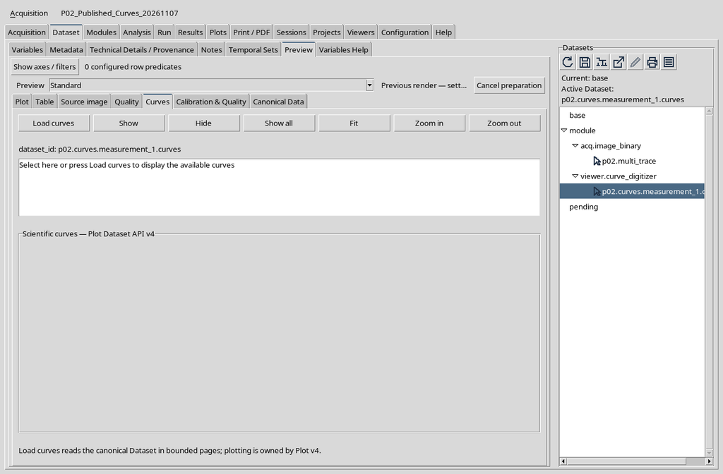
The initial emptiness does not prove that the 24 rows are absent: loading the curves must be requested explicitly.
12. Locating Load Curves
The top bar of the tab contains Load curves, Show, Hide, Show all, Fit, Zoom in and Zoom out. The first command is needed to prepare the scientific representation.
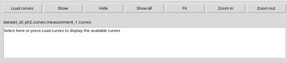
The visibility and navigation commands make sense after the curves have actually been loaded. Their detailed use will be explained in the next chapter.
13. The Initial Message Is a Placeholder
The sentence Select here or press Load curves to display the available curves is not the name of a curve. It is an instruction text and does not correspond to additional scientific rows.
You can press Load curves directly. There is no need to select the placeholder or look for a new file to import: the source Dataset is already the one chosen in the GX-TXT browser.
14. Starting to Load the Curves
Press Load curves. The module requests from the CORE a representation of the canonical data through its cache, without opening a new CSV file manually. The work may be asynchronous: during preparation, do not interpret a temporarily empty panel as a definitive error.
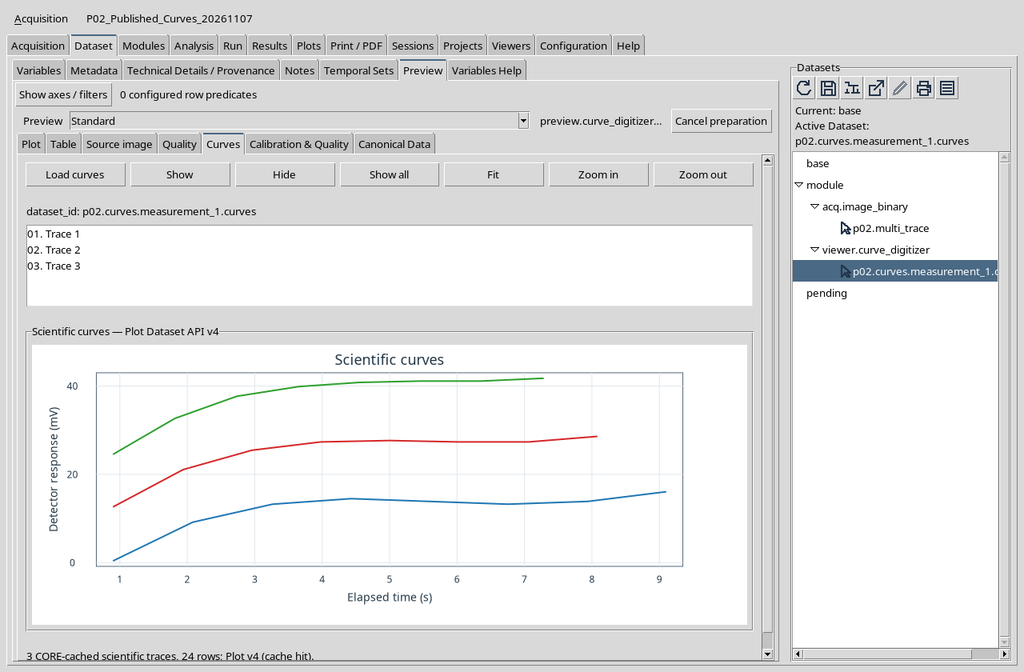
The operation concerns consultation. It is not a digitizing command and does not republish the curves in the CORE.
15. The List Represents the Available Traces
After loading, the list contains three entries. In the documented installation the names shown are Trace 1, Trace 2 and Trace 3. These entries identify the three traces presented by the plot, not new Datasets.

To distinguish the series stably on the scientific level, refer to the identities and names kept in the canonical data, not only to the number displayed in the list.
16. Reading the Native Plot API v4 Graph
The lower part hosts the plot created through Plot Dataset API v4, with axes, tick marks and real series. It is not an illustrative image built separately, nor the source raster.
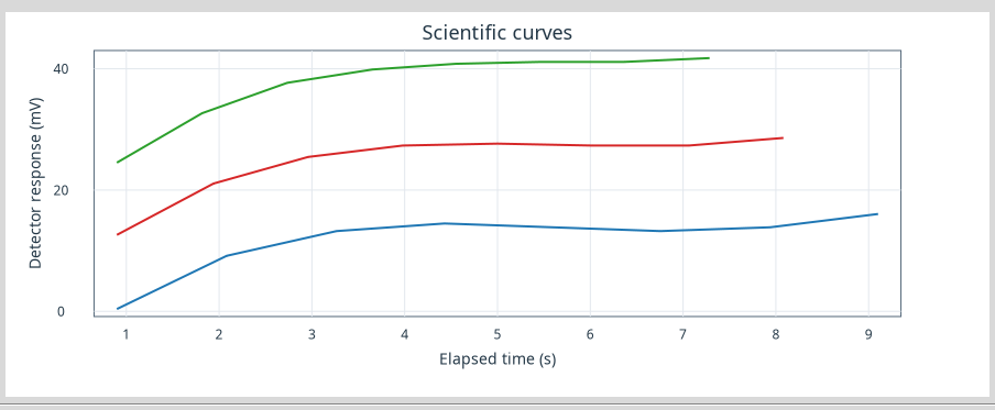
The presence of three lines corresponds to the three published series. Their colours are a representation choice; the scientific coordinates derive from the calibration and the canonical points.
17. Horizontal Axis: Time
The X axis is labelled Elapsed time (s). The number shown along the axis is a physical coordinate in seconds, not a pixel column and not the progressive index of a sample.
When comparing the plot with the source, remember that the point selected on the raster has been transformed by the calibration. A later Zoom in on the Plot does not redefine the second or the original measurement.
18. Vertical Axis: Detector Response
The Y axis is Detector response (mV). The values of the three curves are placed on the same physical scale: in this demonstration a second Y axis with different units is not active.
The vertical position of the original raster has been converted into mV. The scientific plot must not be read as if the vertical screen coordinate were a measurement in itself.
19. Three Curves, Twenty-Four Points
The canonical Dataset contains 24 rows, divided into three curve identities with eight points each. The Preview responds to Load curves with three traces, without losing the original information associated with the individual points.
The graphical connection between the points is a visualization operation. It does not constitute a new fitting, does not generate intermediate values and does not imply an automatic estimate of uncertainty.
20. What Plot v4 Means
The pane shows Scientific curves — Plot Dataset API v4. The plot is managed by the framework’s native engine, which receives a visualization model derived from the CORE Datasets.
The Load curves command prepares the data for the Plot and uses the canonical references of the selected Dataset. The visualization is distinct from the digitization document, from its raster and from the persistent table.
21. Reloading the Visualization
Pressing Load curves again, the tab can reuse a representation already prepared. In the example the status message confirms a cache hit and the panel still shows the same three lines and the same 24 points.
The cache improves consultation, but it does not create a new Dataset. If the source or the Session changes, the representation relating to the identity actually current must be used.
The plot after a second Load curves coincides with the one obtained at the first loading, so there is no need to repeat the same screenshot. To verify the result, check the Dataset ID, the three entries in the list and the Plot axes; a cache hit does not add rows to the canonical Dataset.
22. Canonical Names Remain Distinct from Plot Labels
The curves were published with the names Bias -2 V, Bias -1 V and Bias +0 V. In this version of the Preview, however, the Curves list shows the generic names Trace 1, Trace 2, Trace 3 even after a second loading.
This is a presentation discrepancy to bear in mind: the three series, their names and the points remain in the canonical Dataset. Do not use the text Trace 1 as the persistent scientific identity of the first curve.
23. Loading Does Not Modify the Published Data
Load curves is not equivalent to Publish. It is possible to reload and navigate the plot without creating another publication, altering the source image or rewriting the numerical table.
For a rigorous check, compare the identity of the Dataset and the number of rows before and after the visualization. In this case the Dataset remains the same, with 24 points, without replacements and without new generated curves.
24. Comparing the Representation with Source Image
The Source image tab keeps the distinction between the original raster and the points of the published curves. In the example, five traces drawn in the source graph can be seen; only three were digitized in the exercise.
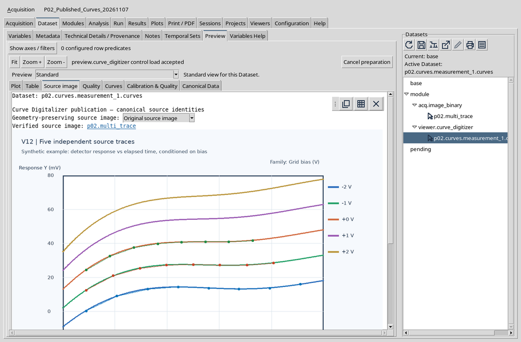
This view makes it possible to find the original context of the points. It does not replace the precision of the calibration, nor does it prove that the non-digitized traces were measured.
25. The Ordinary Plot Tab Is Distinct from Curves
In the same Dataset, the Plot tab of the standard Preview presents a scientific plot. It is useful for general consultation, but it is not the same interface as the Curves contribution, which adds its own list and specialized commands.
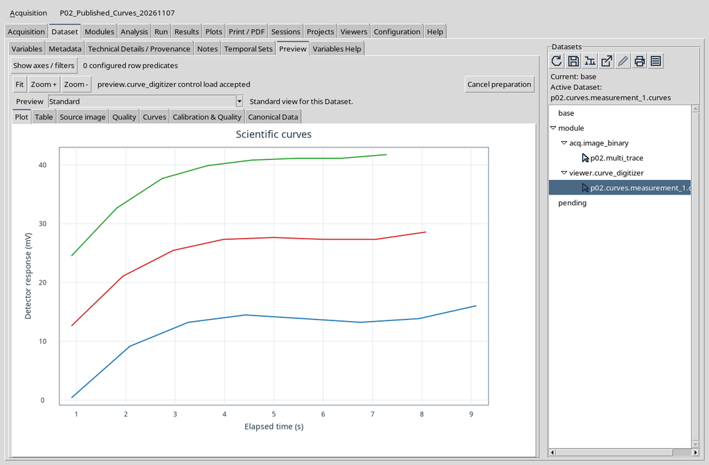
The fact that two tabs show three lines does not mean that there are two publications. The canonical object and its identifier remain unique.
26. Returning to Curves Without Republishing
After consulting Plot or Source image, it is enough to return to the Curves tab. The representation already loaded remains available within the Preview that is still open.
If another Session or another Dataset is chosen, instead, the current identity must be checked before attributing a plot to those data.
Returning to the Curves tab recalls the same representation already illustrated. Reopening a view is not equivalent to Publish selected calibrations: to confirm that there are no new results, look at the Dataset catalogue, not only at the number of curves on the screen.
27. Show, Hide and Show All Are Presentation Commands
The Show, Hide and Show all buttons concern the traces represented on the plot. They should not be confused with Delete curve in the Viewer: hiding a line is not equivalent to deleting its points from the Dataset.
Selecting an entry in the list and comparing visibility with the table will be covered in depth in chapter P03. Do not use graphical changes to infer modifications of the canonical data.
28. Fit and Zoom Are Visual Controls
The Curves tab also shows Fit, Zoom in and Zoom out. They serve to navigate the representation, not to recalibrate the physical axes or modify the coordinates of the points.
The practical effects of Fit and of Plot navigation will be practised in the next guide. For now it is enough to recognize them as controls of the native plot, distinct from the digitizing tools on the raster.
29. Calibration & Quality and Canonical Data
The Calibration & Quality tab is dedicated to the published information on calibration and quality, while Canonical Data allows the rows and scientific variables to be consulted. There is no need to use one of these tabs to make the Plot v4 appear after Load curves.
Their content will be examined separately: a visible curve is a graphical result, but the canonical table and its metadata remain the reference source for scientific analysis.
30. Final Check of the Work
Before using the plot, check in order: the selected Session, the published canonical Dataset, the number of expected curves, the names and units of the axes, the completion of Load curves and the presence of real data in the Plot view.
In our example the results are consistent: three independent curves, eight points per curve, 24 rows, X expressed in s and Y expressed in mV. The only labelling discrepancy observed concerns the generic names in the Curves list, not the published coordinates.
The Dataset Preview therefore makes it possible to move from digitization work to a scientific reading, keeping the distinction between the original source, the registered data and the graphical presentation.