

Dataset Preview — Curve Selection, Show/Hide, Show All, Fit and Zoom
The Curves tab of the Dataset Preview lets you choose which scientific curves to display and navigate the plot through the native Plot Dataset API v4 engine. Selection, visibility and magnification are consultation operations: they do not modify the numerical points registered in the Dataset.
The guide uses a synthetic image with five drawn traces. Three of them are digitized, each with eight points, after a linear calibration. The result is a Dataset of 24 canonical rows, with the X axis in seconds (s) and the Y axis in millivolts (mV). The plot is didactic and does not represent experimental measurements.
1. What the Presentation Commands Are For
When a Dataset contains several curves, it is not always useful to show them all at the same time. You can concentrate on one line, hide it to compare the others or return to the complete view. Show, Hide, Show all and the navigation controls act on the displayed plot, not on the Curve Digitalizer document.
This distinction is essential to avoid a misunderstanding: Hide is not Delete curve, and zoom does not produce new scientific coordinates. The original Dataset remains available to the other GX-TXT functions.
2. Preparing a Dataset Containing Genuinely Published Curves
To begin, you need an Image Dataset source associated with the Curve Digitalizer, an accepted calibration, some curves with points and a canonical publication. Seeing several coloured traces in the raster image is not enough.
In the example three independent series were created, called Bias -2 V, Bias -1 V and Bias +0 V. The points were acquired in the Viewer Canvas; the two remaining traces on the image are not part of the numerical Dataset.
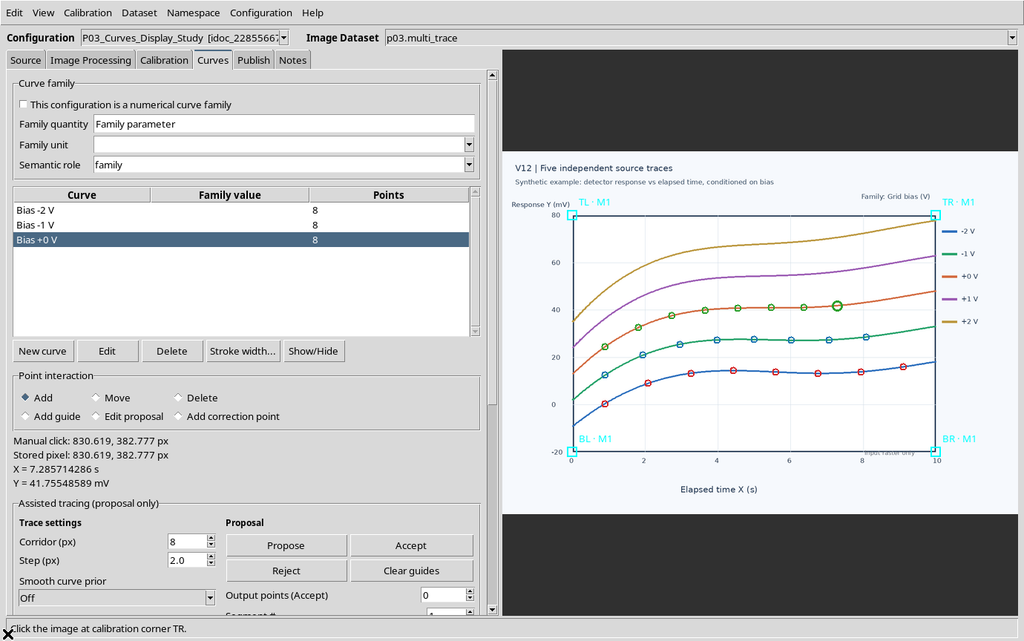
3. Publishing the Curves Before Consulting Them
The Publish tab creates the numerical Dataset in the CORE. For the example an accepted calibration was selected, with separate mode, and publishing completed successfully.
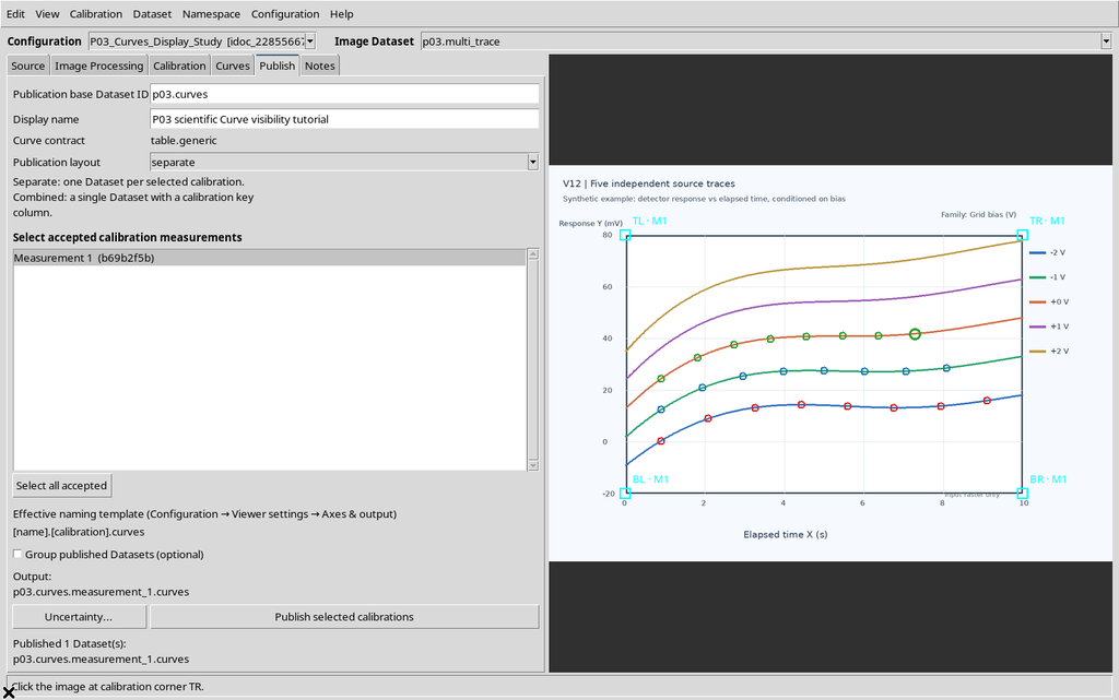
The new Dataset does not replace the source image: both are distinct objects that can be consulted from the Session. Do not repeat Publish to use the visibility buttons.
4. Choosing the Numerical Dataset, Not the Source Raster
In the main GX-TXT window open Dataset → Preview and select the numerical Dataset just published in the Datasets panel. The browser also shows the original source, but that is an image-type object.
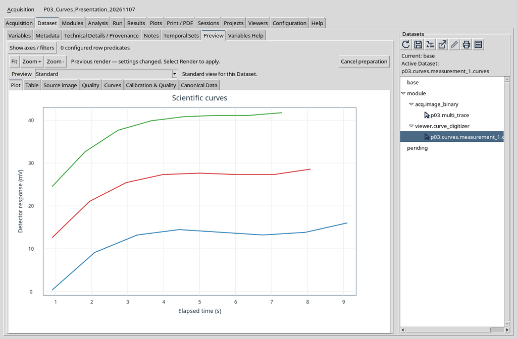
The Preview contains several views of the same Dataset: Plot, Table, Source image, Quality, Curves, Calibration & Quality and Canonical Data. Here we will work only on the Curves tab.
5. Opening Curves When the Plot Is Not Yet Loaded
Select Curves. On first access the plot pane may be empty and the list shows an instruction sentence. This is not an error: the module is waiting for the request to prepare the data to be represented.
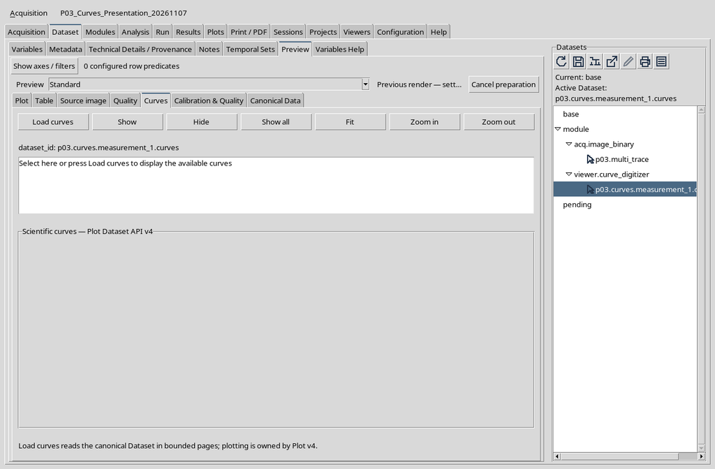
6. Using Load Curves to Load the Plot
Click Load curves. GX-TXT consults the canonical Dataset, prepares the series and shows them through the native Plot v4 renderer. The tab does not import a second raster and does not create another publication.
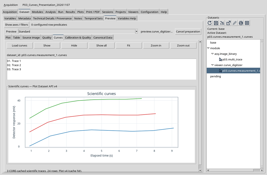
In the example three lines can be seen: one blue, one red and one green. They are representations of the three published numerical series, not photographs of a graph.
7. Locating the Command Bar
Above the list the commands Load curves, Show, Hide, Show all, Fit, Zoom in and Zoom out appear. The first four control preparation and visibility respectively; the last three change the framing of the Plot.
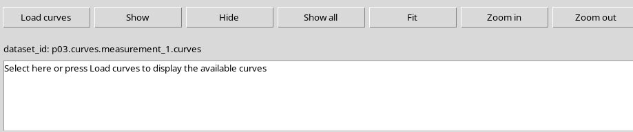
It is important to distinguish these buttons from the similar tools in the Viewer: here you operate on data already published; you do not acquire points from the raster.
8. Understanding the List of Curves
Below the Dataset identifier a list with three entries appears: 01. Trace 1, 02. Trace 2 and 03. Trace 3. The numbering indicates the traces of the plot and not the global order of the rows in the scientific table.
The original names Bias -2 V, Bias -1 V and Bias +0 V are kept in the Dataset. In this version of the Preview contribution, however, the list uses generic Trace N labels. To recognize a series persistently, refer to the name and the canonical identity of the curve.
9. Selecting the First Row with the Mouse
Click 01. Trace 1 in the list. The selected row is highlighted; the plot continues to show all the curves until one of the visibility controls is invoked.
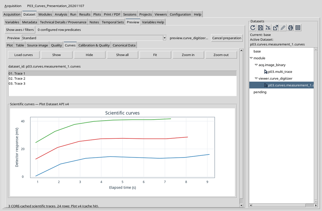

The selection establishes which series Show or Hide will act on. On its own it does not change the number of points.
10. Hiding a Single Curve with Hide
With the first row selected, click Hide. The blue line disappears from the Plot, while the red and green lines remain visible.
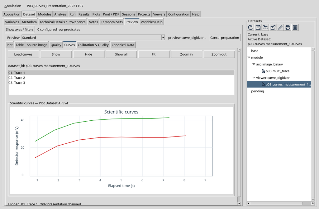
The status message reads Hidden: 01. Trace 1. Only presentation changed. It is a change of visibility, not a deletion from the Dataset.
11. Checking That the Other Two Curves Do Not Change
The disappearance of the first line must alter neither the position of the other curves nor the scientific scale in use. You can continue to compare the red and green lines while keeping the same axis system.
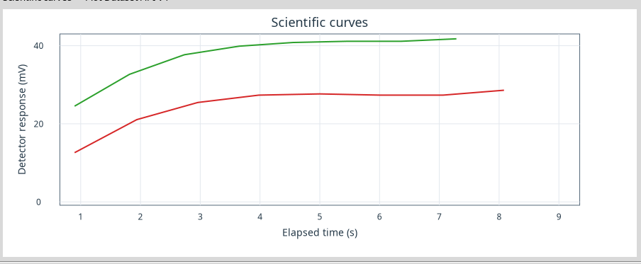
The first curve continues to exist in the Dataset and can be displayed again without rerunning the Curve Digitalizer.
12. Restoring the Selected Curve with Show
With the first row still selected, press Show. The blue line returns to its place and all three series are visible again.
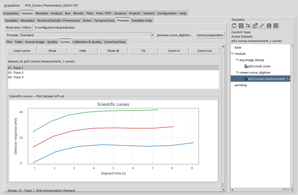
The result corresponds to the same three-curve view available before the Hide operation.
13. Moving to the Second Curve
Click the entry 02. Trace 2. It is the second row of the native list and, in the example, corresponds to the red trace.
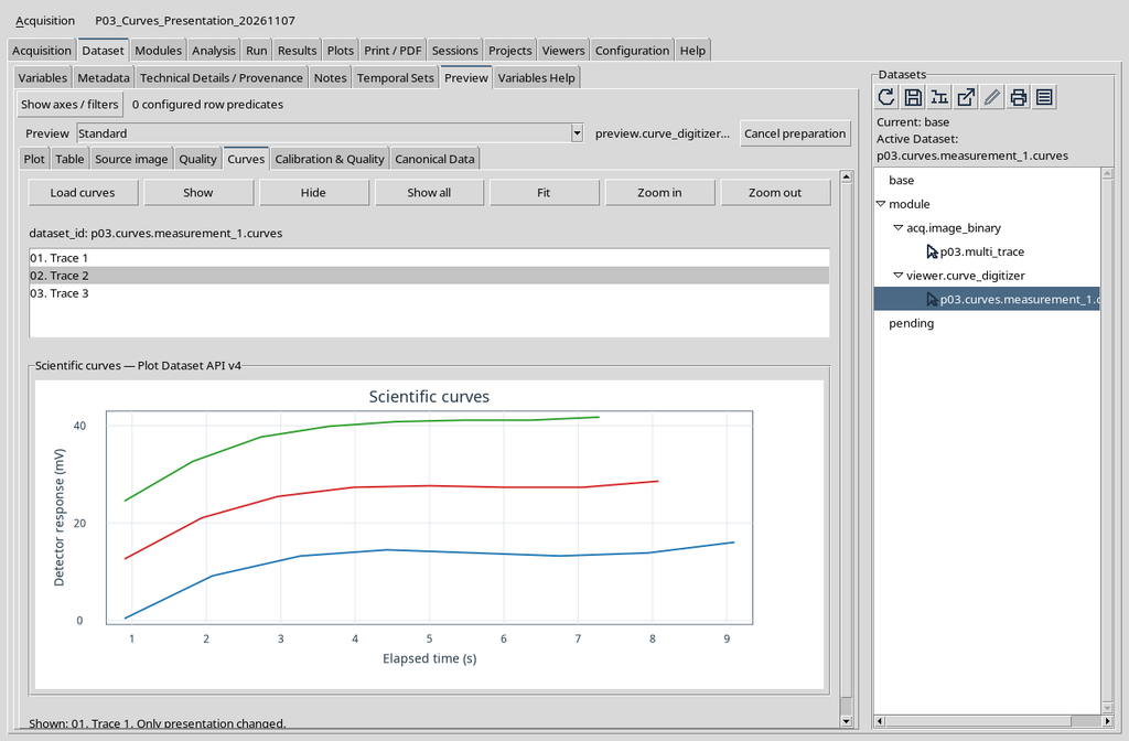
The selection is not equivalent to a filter on the canonical data: it simply determines which trace is the target of the next Show/Hide action.
14. Hiding the Second Curve
Press Hide with the second row selected. The plot leaves the first blue line and the third green line visible, while the red one is no longer drawn.
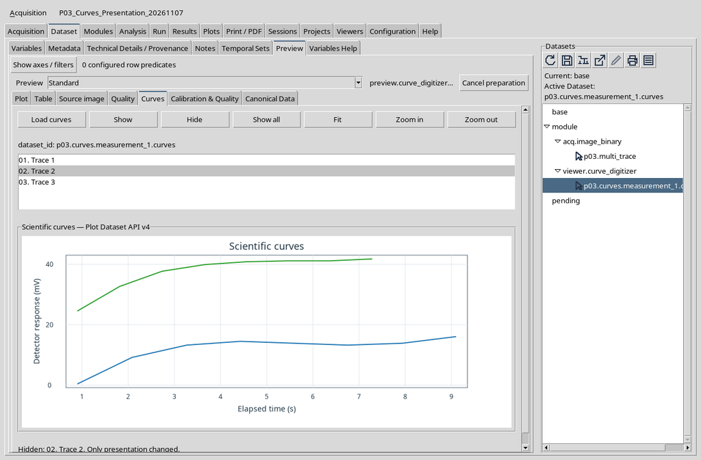
The result shows that visibility is controlled per individual series, not for the whole Dataset.
15. Restoring All the Lines with Show All
To show all the series at the same time, press Show all. There is no need to clear the previous selection or to act directly on the Dataset.
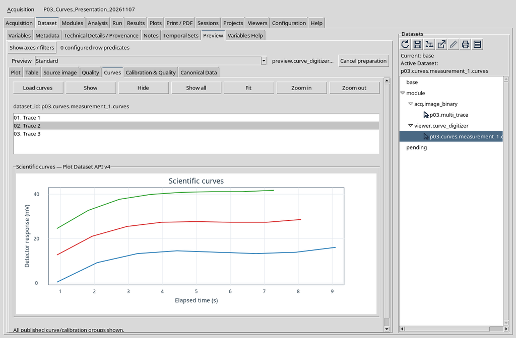
The command is useful when one or more curves have been temporarily hidden and you want to return to a complete representation.
16. Selecting the Third Curve
Click 03. Trace 3. The row corresponds to the green trace in the example, while the first and second remain visible.
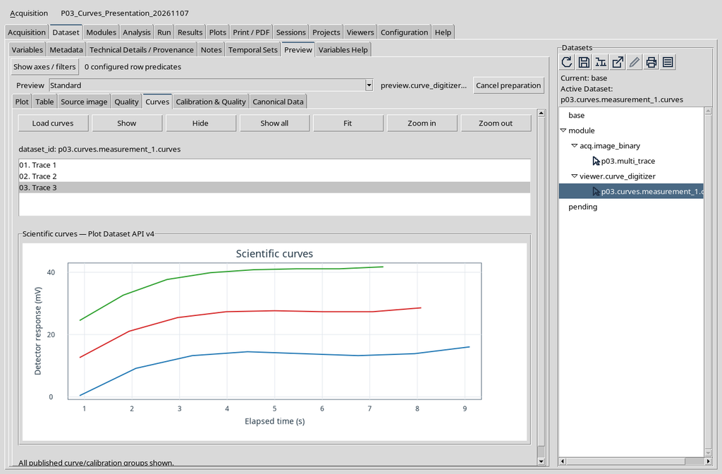
Selecting the third entry does not change the order of the points and does not reassign the names or scientific identifiers of the other curves.
17. Hiding the Third Curve
Press Hide after selecting the third entry. Now only the blue and red lines are visible.
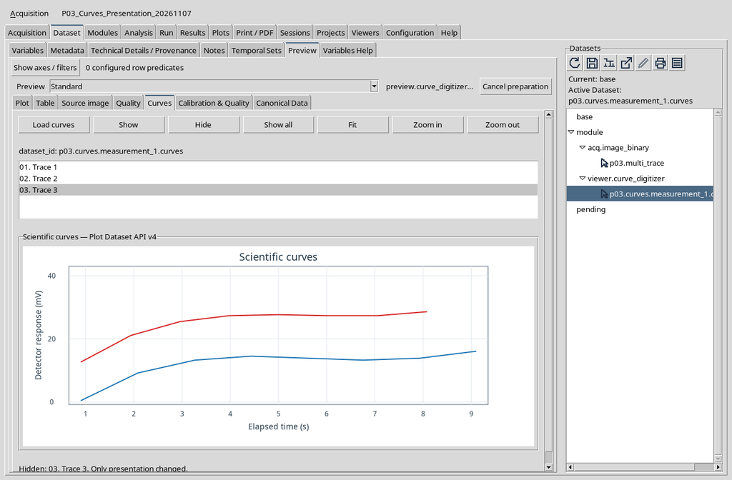
In ordinary work this procedure can be repeated to visually isolate the part of the plot of interest, keeping the presentation criterion distinct from the structure of the Dataset.
18. Returning Once More to Show All
Press Show all. All the curves become visible again. The result does not require Publish, does not insert new points and does not change the number of rows.
After hiding the third trace, press Show all to restore the visibility of all the curves in a single step. The command does not depend on the row currently selected: it acts on the set of loaded traces.
The final representation coincides with the previous complete one. No new acquisition of points is needed and no Dataset is created: the same 24 canonical rows remain in the Session.
19. The Difference Between Hide and Deletion
In the Curve Digitalizer the command to delete a point or a curve changes the editable scientific document; a subsequent publication can therefore produce different data. In Dataset Preview, instead, Hide and Show act on a representation that has already been prepared.
For this reason the Hide command must not be used as if it were a table clean-up operation: data excluded only from the view are still present.
20. The Canonical Rows Remain Twenty-Four
Throughout all the selection, Hide, Show and Show all tests, the published Dataset kept the same 24 rows, with the same identifiers and contents. The digital identity of the numerical content was also verified before and after the visibility changes.
This check distinguishes a visual effect from a transformation of the data: the plot can show one, two or three lines without the Dataset having to be rewritten.
21. What Fit Represents
Fit adjusts the view of the plot to bring the entire scientific range of the loaded series back into the frame. It is a navigation command, not the fitting of a function to experimental data.
The name can be misleading: Fit in the context of the Plot means adjusting the framing. It does not generate a regression, does not calculate new coefficients and does not modify the points.
22. Magnifying with Zoom In
With the three curves visible, press Zoom in. The native engine narrows the scientific ranges shown on the axes, focusing on the central part of the plot.
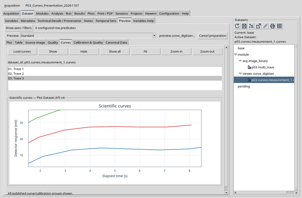
Magnification does not change the units: the X axis remains expressed in seconds and the Y axis in millivolts.
23. How the Scientific Ranges Change
In the case reproduced, the visible X range narrows from about 0.652–9.348 s to 1.521–8.479 s; the Y range goes from about −0.865–42.997 mV to 2.832–37.922 mV.
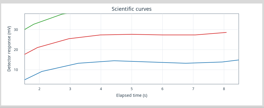
These are view limits, not extremes measured with a new calibration. The values depend on the Dataset displayed and on the current framing.
24. Reducing Magnification with Zoom Out
Press Zoom out to widen the visible portion of coordinates again. In the example, after a single Zoom in and a single Zoom out, the limits return practically to the starting ones.
The command does not add points at the edges of the curve: it makes areas of the range already belonging to the representation observable again.
To verify the result of Zoom out, read the numerical limits of the axes before and after the command. In the example the visible range returns to about 0.652–9.348 s for X and −0.865–42.997 mV for Y, as shown in the comparison table.
If the Plot displays all three curves again, this is the same scientific representation, not a republication. Recovering the complete view does not alter the calibration or the stored values.
25. Using Fit to Restore the Axes
After one or more changes of magnification, Fit lets you return to a complete view consistent with the available data. In the test carried out, the initial axis limits were restored.
Fit can be useful before comparing two curves or before moving to another Dataset, avoiding interpreting a magnified detail as the whole phenomenon.
Fit is useful above all when zoom has been repeated several times or the framing no longer includes the entire data range. After pressing it, check that the three traces are fully visible again and that the axis units are still s and mV.
In the case described here, the final screenshot coincides with a complete view already illustrated: the quantitative comparison is in the following section. The Fit command adjusts only the scale of the plot and does not perform a mathematical fitting of the curves.
26. A Numerical Comparison of the Three Views
| Operation | Visible X range | Visible Y range |
|---|---|---|
| Before zoom | about 0.652–9.348 s | about −0.865–42.997 mV |
| Zoom in | about 1.521–8.479 s | about 2.832–37.922 mV |
| Zoom out | about 0.652–9.348 s | about −0.865–42.997 mV |
| Fit | about 0.652–9.348 s | about −0.865–42.997 mV |
The limits represent ranges returned by the native Plot in the screenshots examined, rounded for convenience. The table describes the framing, not the uncertainty of the points or a new measurement.
27. Difference Between Raster Zoom and Plot Zoom
Zoom in the Curve Digitalizer serves to work with the source image and the pixel positions. Zoom in Dataset Preview → Curves, instead, acts on the scientific coordinates already published, expressed in the units of the axes.
Confusing these two levels can lead to interpreting a change of magnification as a change in the data. The relationship between pixels and units is fixed by the original calibration, not by the Preview navigation buttons.
28. Series Names Are Scientific Data, Not Colours
The blue, red and green colours are useful to distinguish the traces visually, but they do not constitute a canonical identifier. Nor should the generic label Trace 1 replace the name of the published series.
For later uses — processing, export, comparison between Sessions and reproducibility — use the identities and names present in the scientific Dataset. In this version the Curves list retains the presentation discrepancy already reported in chapter P02.
29. If the Plot Does Not Match the Expected Curves
First check the Session, the identifier of the chosen numerical Dataset, the presence of the published curves and the completion of Load curves. If the view contains fewer lines than expected, check whether some have been hidden and try Show all.
If the framing is too narrow, use Fit before suspecting missing points. Do not republish the Dataset, do not replace the source and do not modify the calibration to solve a simple presentation condition.
30. Summary of the Operations
The essential sequence is: Dataset → Preview → select the numerical Dataset → Curves → Load curves → choose a row → Show or Hide. Show all restores the lines, Zoom in and Zoom out change the observed range, Fit returns a complete view.
In the example all the actions left the 24-row numerical Dataset, the original source and the physical units of the axes unchanged. The presentation is reversible; the published scientific data remain independent of visibility and magnification choices.