

Dataset Preview — Comparing Views, Publications and Scientific Axes
The GX-TXT Dataset Preview offers several representations of the same scientific content: a raster source, a numerical table, a plot and, when the Dataset was produced by the Curve Digitalizer, specialized tabs for curves, calibration, quality and traceability. This guide helps you recognize them and choose the appropriate view without confusing what you see with what is actually registered.
The examples use synthetic graphs and Datasets belonging to different Sessions and configurations. They must therefore not be interpreted as repeated measurements of the same experiment. For each comparison the relevant conditions are declared: Dataset type, number of points, calibration and physical units.
1. Which Preview Are We Consulting?
The framework’s Dataset → Preview tab is one thing; the views offered within it are another. The ordinary display is also available for a raster, while the specialized Curves, Calibration & Quality and Canonical Data tabs require a compatible numerical publication from the Curve Digitalizer.
To interpret a screenshot correctly, always check the Session, the Active Dataset, the Contract and the selected tab. The presence of a Plot button or of a plot on the screen does not, on its own, guarantee that published canonical data exist.
2. State A — A New Session May Contain No Datasets
Open a Session without imported Datasets and choose Dataset → Preview. The initial state may show a message about the absence of a readable CSV file and indicate Active Dataset: None.
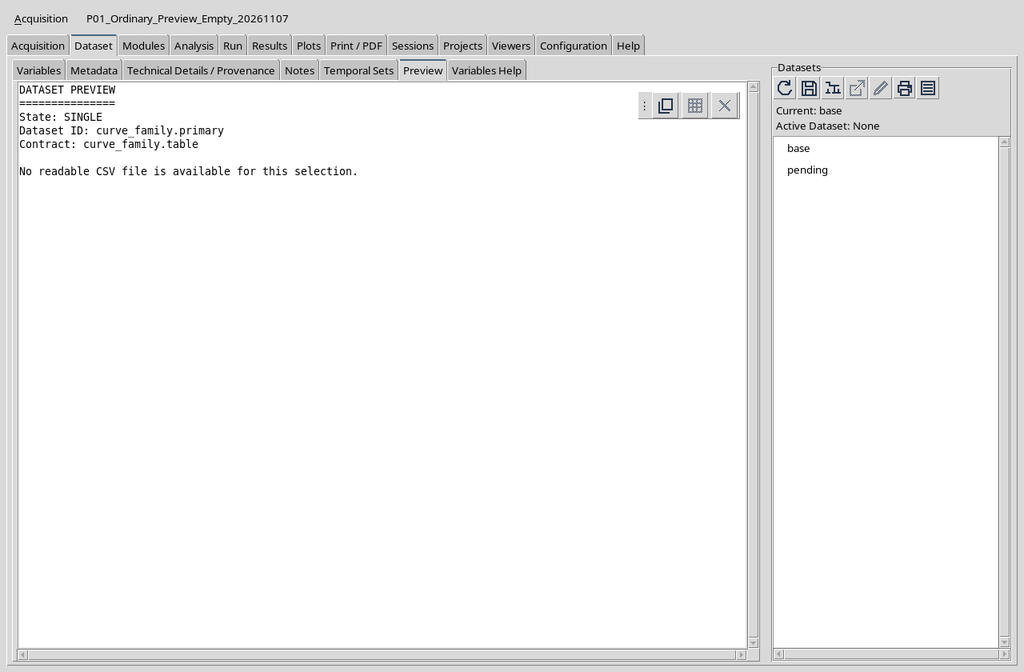
The message does not concern the scientific quality of a curve: there is not yet any publication to compare. For this state it is inappropriate to speak of physical axes, numerical points or validated calibration.
3. State: SINGLE Does Not Mean “Single Published Curve”
The State: SINGLE label concerns the input selection mode. In the state without CSV, values shown such as Dataset ID and Contract may be default settings: they do not necessarily represent a Dataset present in the Session catalogue.
Before inferring anything from a header row, check the Datasets browser and the actual content of the selection. A placeholder is not an original numerical row.
4. State B — The Original Raster Is an Image Dataset
After importing a compatible image file, the ordinary Preview can represent the original raster. You see pixels, figures and graphical annotations, not necessarily scientific abscissas and ordinates already digitized.
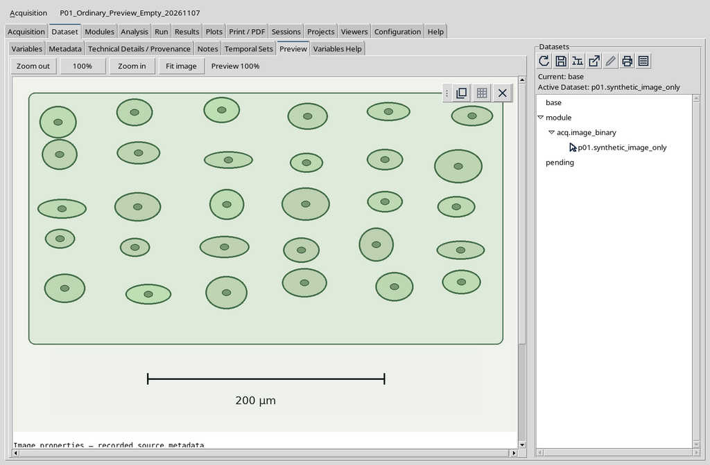
In this view, Zoom in, Zoom out and Fit image change the presentation scale of the pixels. They do not insert points and do not convert the image coordinates into scientific measurements.
5. State C — A Published Numerical Dataset Is a Different Object
The Curve Digitalizer transforms the points acquired on the raster through a calibration and, after Publish, registers a canonical Dataset in the CORE. In the browser the image source and the numerical result are distinguished.
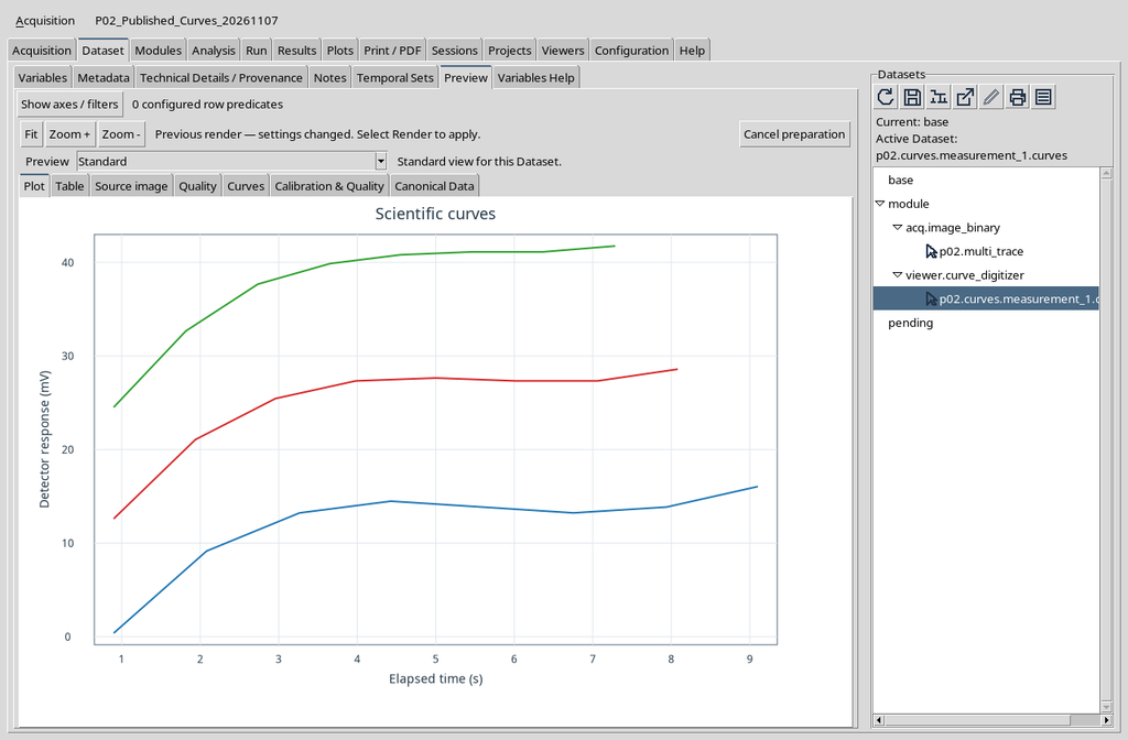
A table.generic Dataset has rows and declared variables; the image.raster has pixels and source properties. Do not treat them as if they were interchangeable.
6. The Curves Contribution Need Not Be Already Loaded
After choosing a compatible numerical Dataset, the Curves tab may be present and initially empty. Its message invites you to use Load curves.
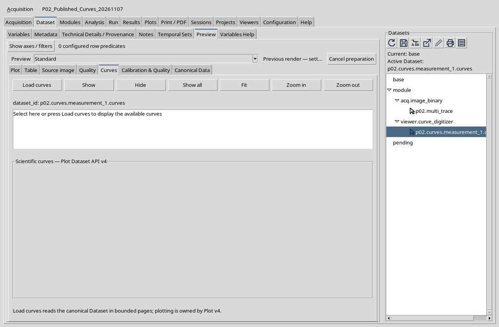
This state does not prove that the data are absent. The Dataset is already registered; the module has not yet prepared the graphical representation.
7. Load Curves Makes the Scientific Plot Visible
Press Load curves to display the numerical series through Plot Dataset API v4. In the example the result contains three curves, each with eight points, for a total of 24 rows.
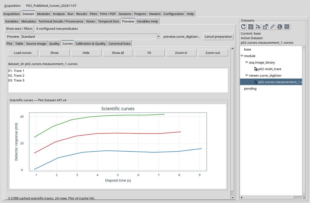
This is a plot produced from the published data, not a photograph of the source. The number of traces is not the number of Datasets: three curves can belong to a single Dataset.
8. Ordinary Plot and Additional Curves Are Not Two Publications
The standard Plot tab and the additional Curves tab can show the same numerical series through different interfaces. Curves adds a list and visibility buttons; the standard Plot offers the general display.
Before comparing two plots, check that they point to the same Dataset and have compatible axes, units and ranges. Two graphically similar images do not by themselves prove row and calibration identity.
9. Hide Changes Visibility, Not the Dataset
In the Curves panel select an entry and press Hide. One line disappears from the plot; the others continue to be represented.
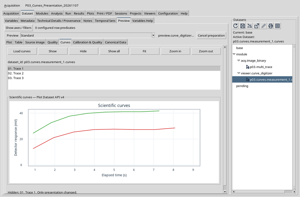
Hide does not delete the Point ID, the numerical row or the original image. In a separate check, the identifiers and the digital fingerprint of the Dataset remained unchanged.
10. Show All Restores the Visual Comparison
Press Show all to bring the lines back into the representation. It is a reversible action that does not require a new publication.
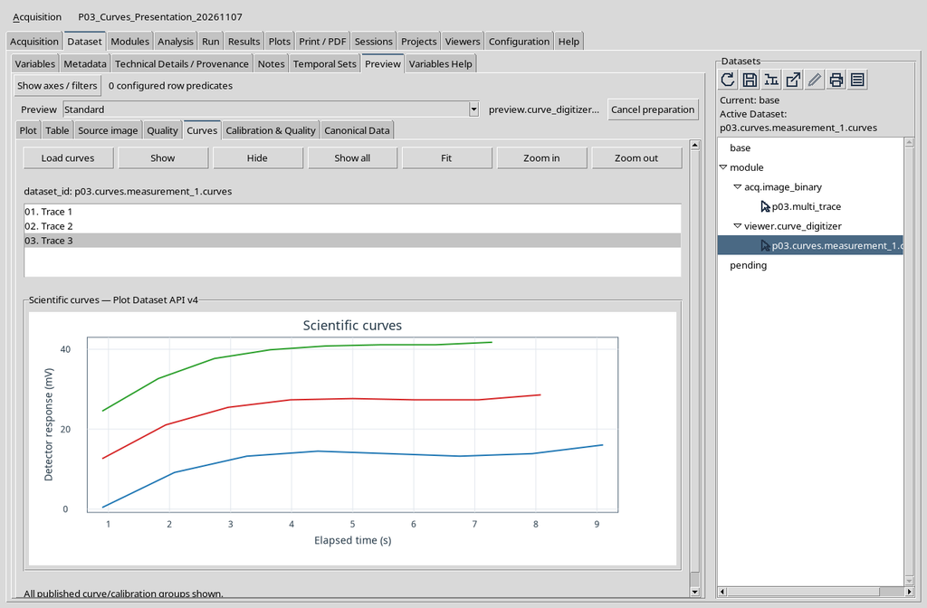
For a scientific comparison, temporarily hiding curves can help reading, but it must not be presented as an irreversible filter applied to the data.
11. Calibration & Quality Exposes Publication Metadata
The Calibration & Quality tab summarizes origin, units, calibration realizations, counts and diagnostics associated with the numerical Dataset.
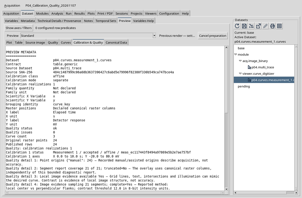
The Source Dataset and Source SHA-256 fields make it possible to verify the identity of the source. The calibration fields describe what was published, not a new physical measurement.
12. Quality “ok” Does Not Prove Physical Accuracy
In the example the published report indicates Quality status: ok, Quality issues: 0 and 24 manual points, but distinguishes Accuracy status: not_assessed from Uncertainty status: not_declared.
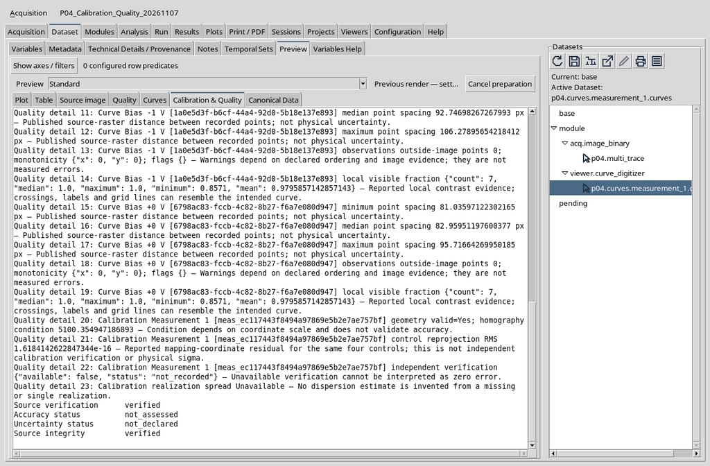
Even a numerical reprojection very close to zero on the four controls used for the calibration does not replace an independent verification. An undeclared uncertainty must not be treated as zero.
13. The CORE Quality Tab Has a Different Structure
The standard Quality view presents the data in a table with the columns Diagnostic, Value, Unit and Meaning. It is useful for consulting the explanation associated with a single indicator.
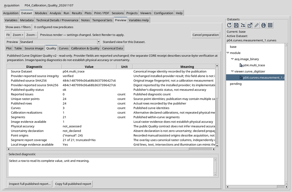
The content comes from the published report; the table layout does not create a second analysis. Here too it is necessary to read the limitations of the fields, not just their value.
14. The Same Identity Can Have Several Representations
The original image, the curves in the Plot, the numerical table and the quality report perform different functions. The first keeps the visual context; the Plot makes the trends visible; the table exposes the values; Quality describes checks and provenance.
A correct workflow uses all the views when necessary, but keeps the canonical Dataset as the reference for numerical processing.
15. Canonical Data May Initially Be Empty
In the Canonical Data tab the first access does not necessarily load rows immediately. The message invites you to press Load to request the first page.
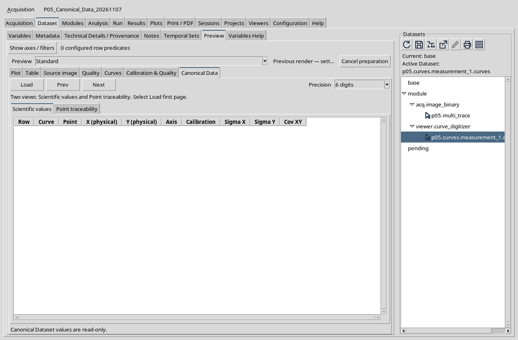
Loading takes place through the CORE services: there is no need to open a separate CSV, guess a column or copy the points from the plot.
16. Scientific Values Shows Numbers and Scientific Roles
In the larger example three synthetic curves with 22 points each were published, that is 66 rows. The first page of Scientific values shows the first 50.
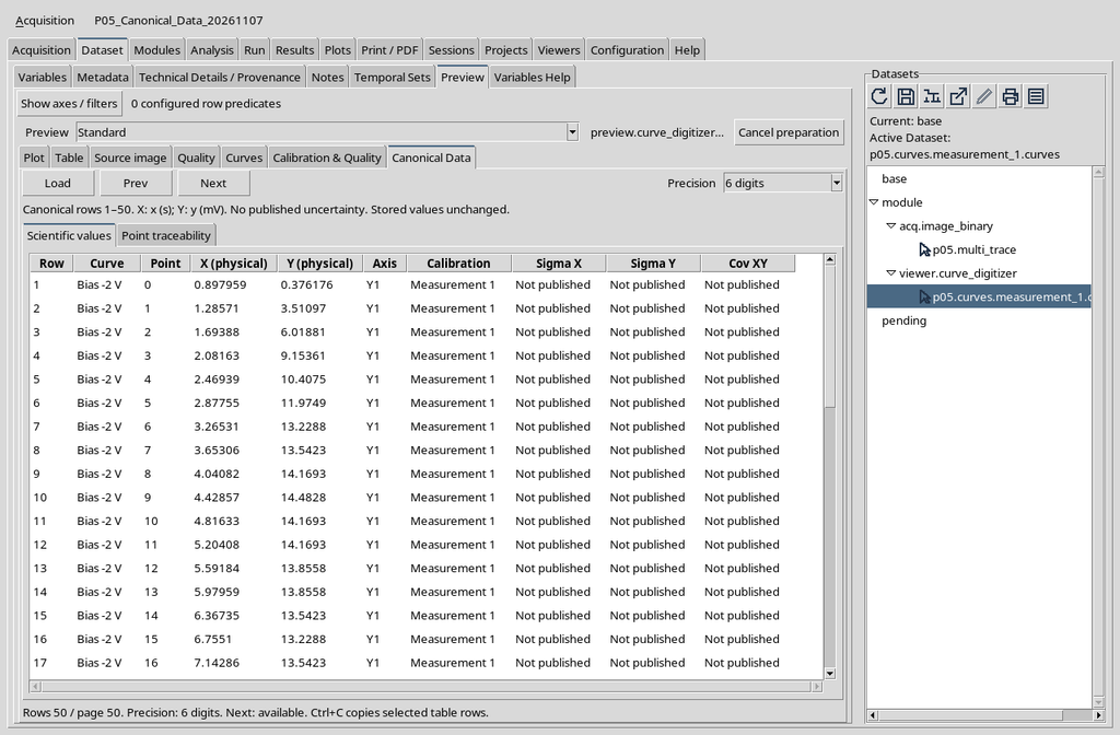
Row identifies the row of the Dataset, while Point represents the order within the curve. X and Y are physical quantities in the declared units.
17. Point Traceability Preserves the Original Identity
The Point traceability view presents Curve ID, Point ID, Calibration ID, Pixel X and Pixel Y for the same rows.
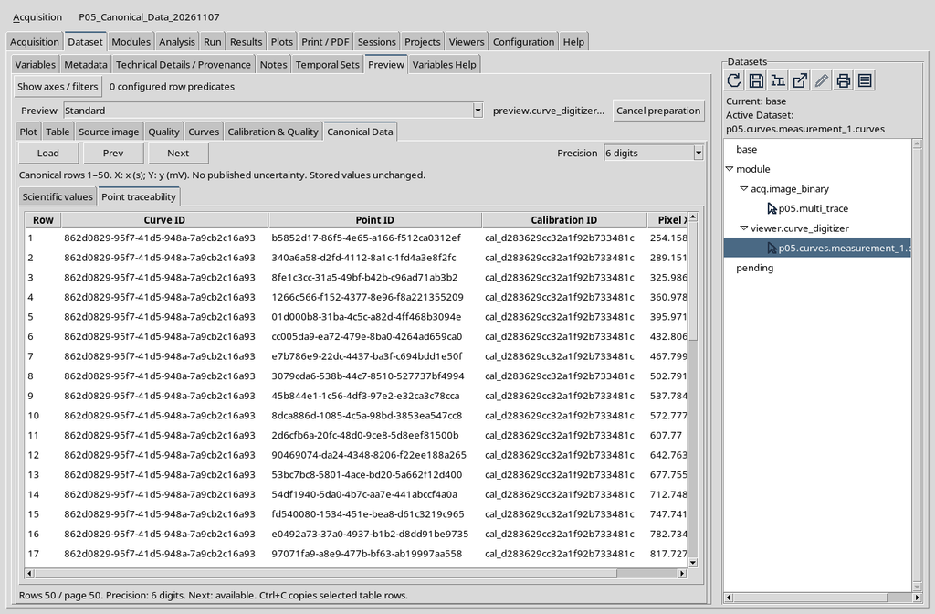
The IDs must not be derived from the colours of the plot. The pixel values must not be confused with abscissas in seconds and ordinates in millivolts.
18. Pagination Is a Property of the View
Pressing Next, in the case of 66 rows, moves from the first 50 to the last 16. The number of canonical rows remains 66.
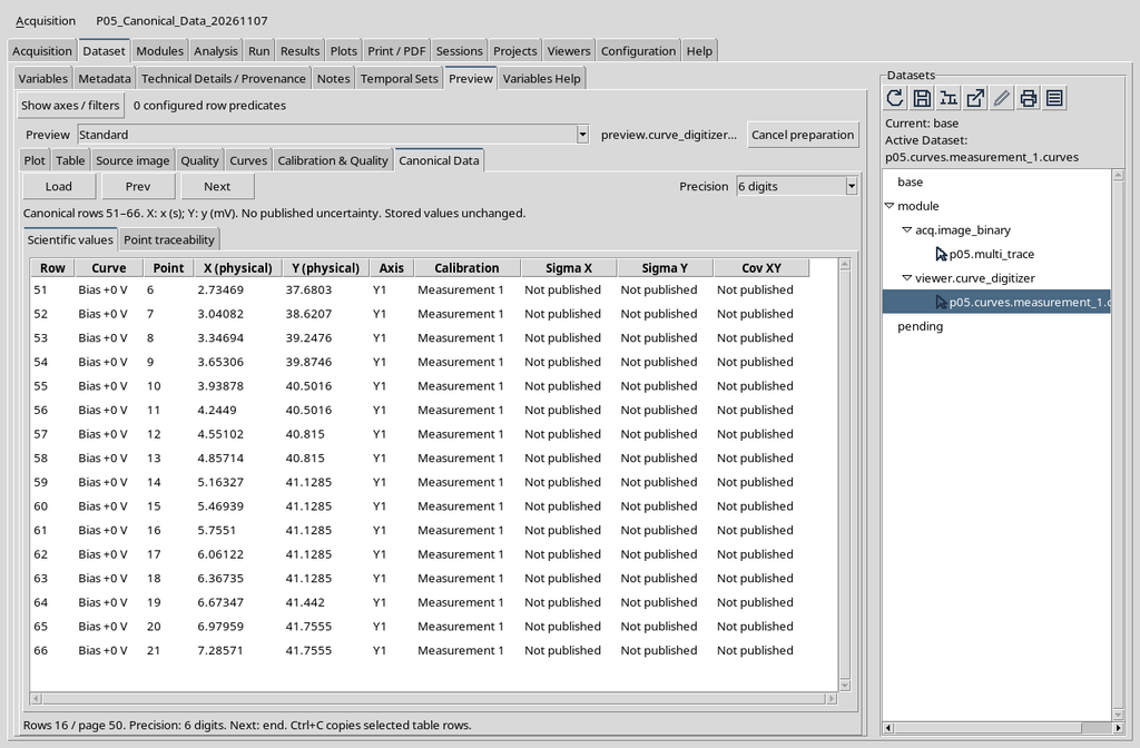
Prev lets you return to the first block. The pagination limits must not be mistaken for missing data or the deletion of a curve.
19. Full Precision Changes How Values Are Printed
The Precision menu offers 6 digits, 10 digits and Full precision. These options change the text representation of the numbers, without altering the persistent values.
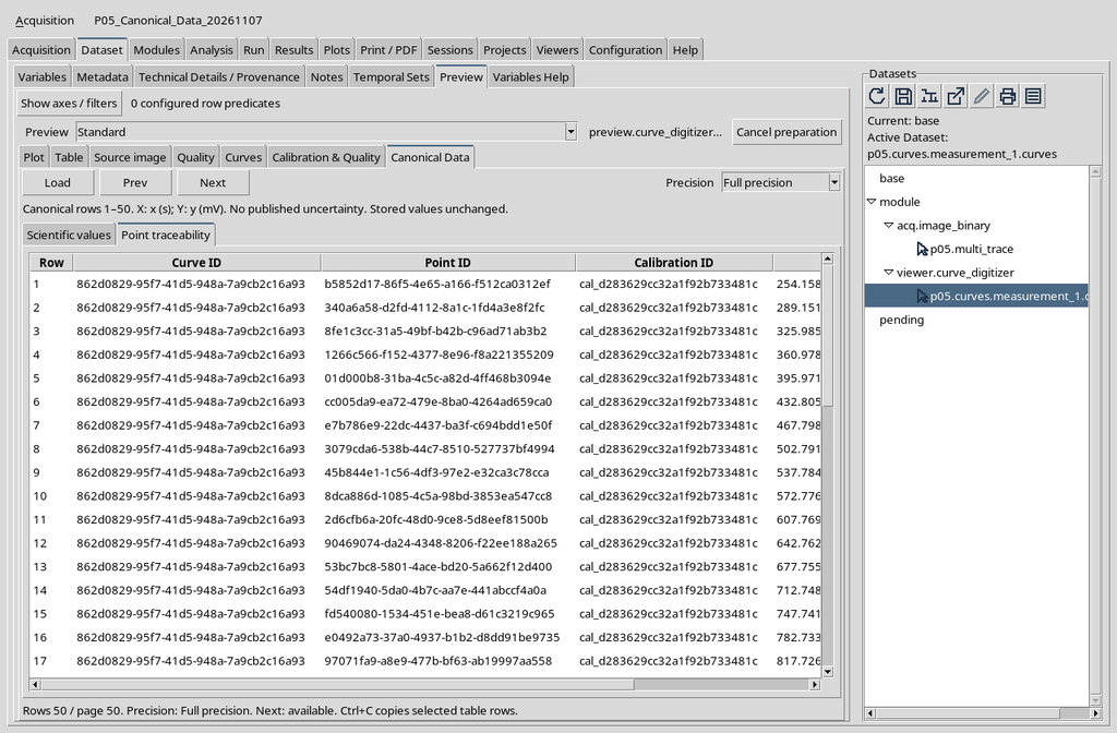
Do not confuse the number of digits shown with experimental accuracy. The Sigma X, Sigma Y and Cov XY columns may legitimately indicate Not published when the uncertainty has not been declared.
20. An Independent Check of the Values Must Use the CORE
A table that appears consistent is not enough to evaluate the integrity of a Dataset. A more rigorous comparison uses the CORE public APIs, for example DATASET_PREVIEW_API_v1, to reread Scientific values and Point traceability and compare the values with those of the selected Dataset.
Pagination and the choice of Precision are consultation operations: they must not rewrite the Dataset. If different Sessions are compared, the identity of the Dataset and the provenance of the source must be checked explicitly, including the SHA-256 fingerprint.
21. Configuration with a Single Y Axis
In the Curve Digitalizer, without a secondary axis, the calibration shows the X and Y axes. Each point is transformed using the physical quantity declared on the single vertical axis.
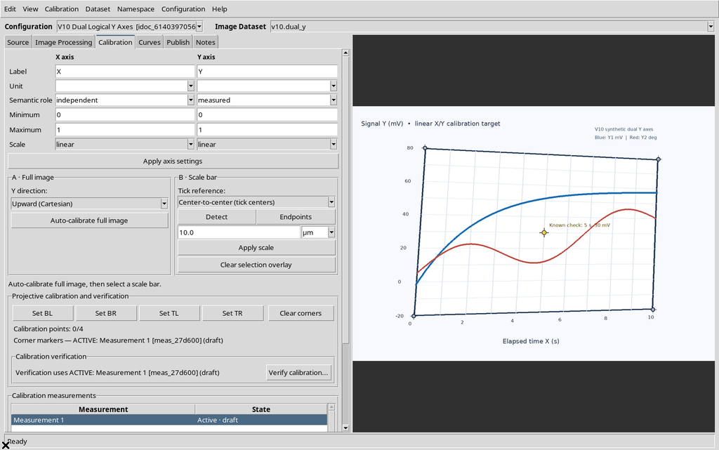
This configuration is suitable when the series share a single Y quantity and do not need to represent a second physical unit.
22. Enabling the Second Logical Axis Y2
The Enable secondary Y axis option, on the Viewer settings page, lets you declare a second independent Y axis. In the case illustrated Y1 represents an amplitude in mV, while Y2 is configured as a phase in degrees.
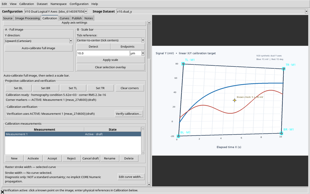
The Y2 axis uses the same geometric references of the raster, but its own scale and scientific unit. The Y2 model must not be interpreted as a simple second colour.
23. Checking X, Y1 and Y2 at the Same Point
The Viewer lets you display the three scientific coordinates relating to the same raster position. The check places the X value, the Y1 value and the configured Y2 value side by side.
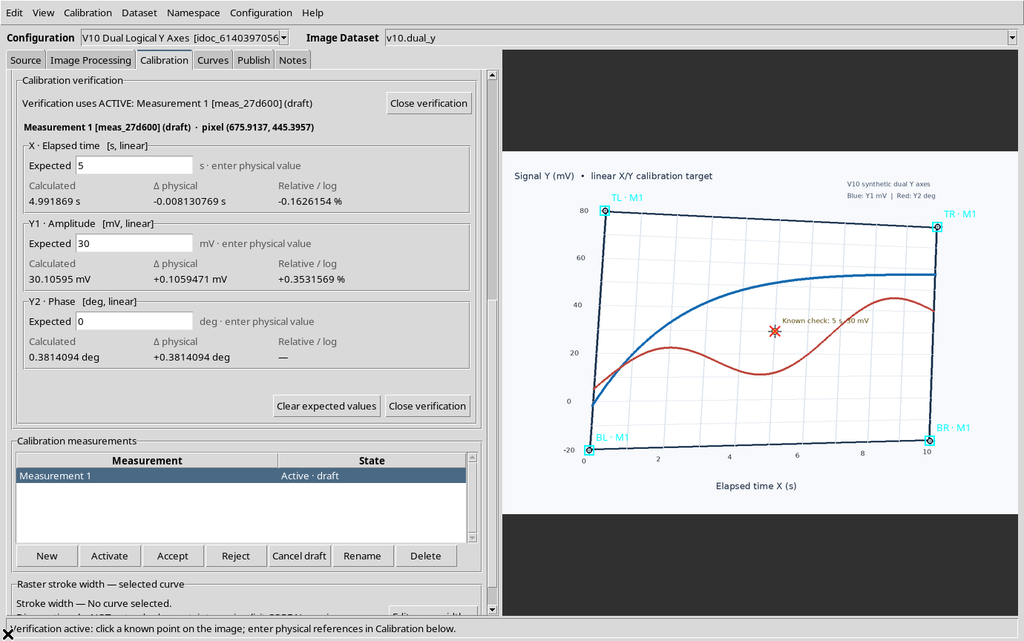
A check of the transformation is not equivalent to an external experiment: physical accuracy requires independent references and an explicit uncertainty model.
24. Assigning a Curve to Y1 or Y2
When Y2 is enabled, the Viewer’s Curves tab exposes the logical association of the series with the appropriate axis. In the configuration example there were two placeholder curves, one associated with Y1 and one with Y2.
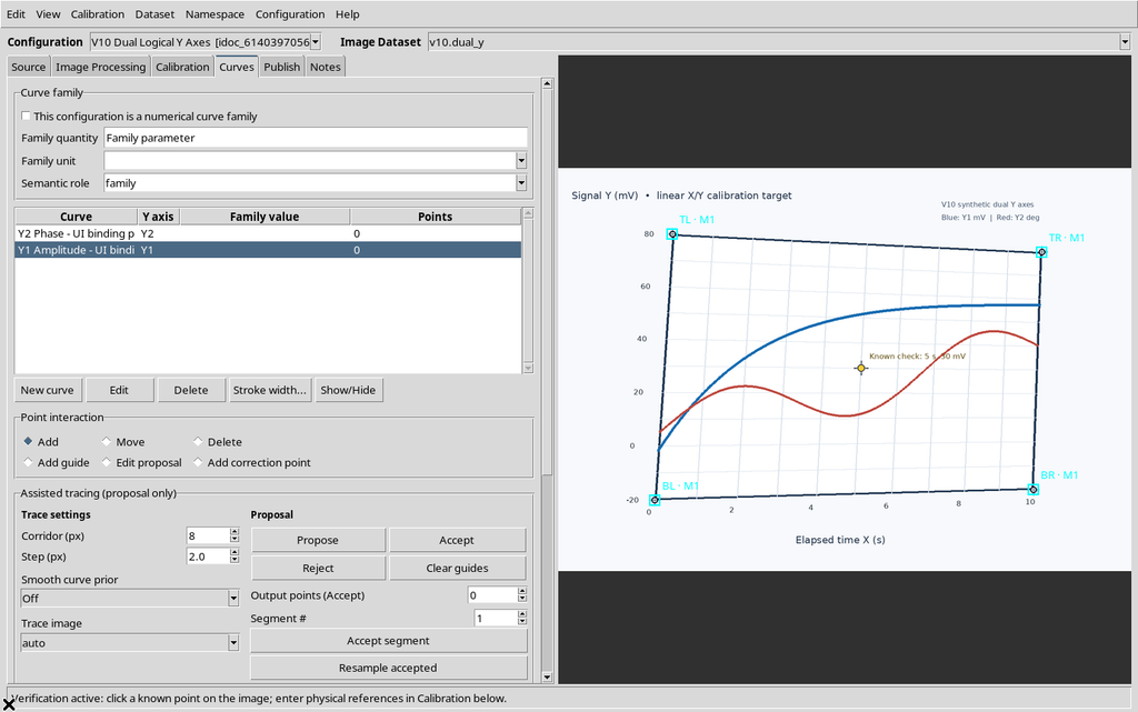
A placeholder curve with zero points shows that the Y1/Y2 selection is available; it does not show that a published dual-axis numerical plot already exists.
25. Distinguishing Dual-Y Configuration from Proof of the Dual-Y Plot
Enabling Y2, checking the coordinates in the Viewer and publishing the data are distinct phases. The presence of a Y2 column in the calibration does not authorize claiming that the additional Curves tab has already rendered two physical axes in the Plot Dataset API v4.
The screenshots illustrated here show the configuration and publication of the Y1/Y2 data and their consultation in the ordinary CORE scientific Viewer. They do not, instead, present an example of the Curves contribution simultaneously reproducing two Y axes with different units through Plot Dataset API v4.
26. Separate — Two Accepted Calibrations, Two Planned Results
The Separate publishing mode keeps the results of two accepted calibration realizations distinct. In the example with Trial A and Trial B, the same ten original points were interpreted with two slightly different geometric transformations.
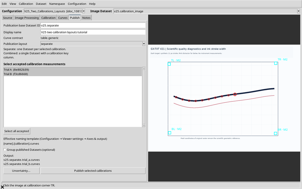
Two publications can share the same raster source and the same Point IDs, but contain different X/Y coordinates because the calibration used does not coincide.
27. Separate — Two Datasets Actually Published
After the publish command, the Viewer registered two numerical Datasets, each with 10 rows. The two outputs keep their own calibration identity separate.
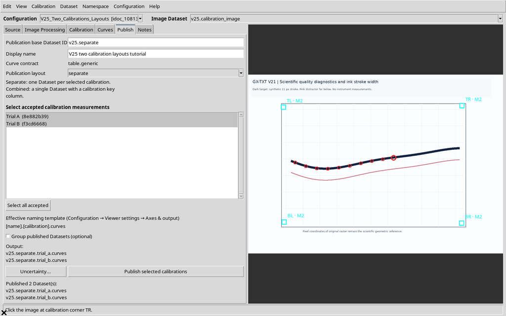
This is a comparison between two transformations of the same points of the synthetic source, not two independent physical acquisitions. The distinction is important when comparing the numbers.
28. Combined — One Planned Output for Several Calibrations
Switching to Combined mode, with the same two realizations selected, the plan proposes a single Dataset containing both sets of coordinates. The Dataset must keep a key identifying the calibration associated with each row.
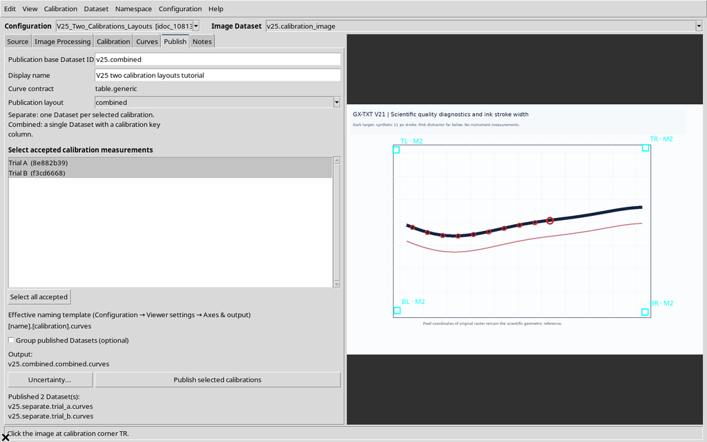
Combined does not mean averaging the two calibrations. It means keeping the realizations inside a tabular container that allows them to be distinguished unambiguously.
29. Why Combined Shows a Warning
When calibration realizations are merged, applications that ignore the calibration key could treat non-equivalent rows as belonging to a single transformation. The GUI explicitly warns of this risk.
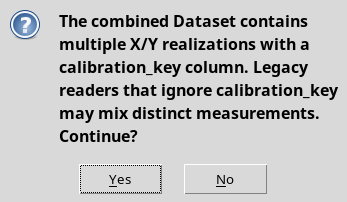
The dialog’s cancel command does not publish the new Dataset. The operation must be confirmed consciously, after checking how the calibration identities will be kept.
30. Combined — A Twenty-Row Dataset
After confirmation, in the example the Viewer publishes a 20-row Dataset, made up of ten rows for Trial A and ten for Trial B.
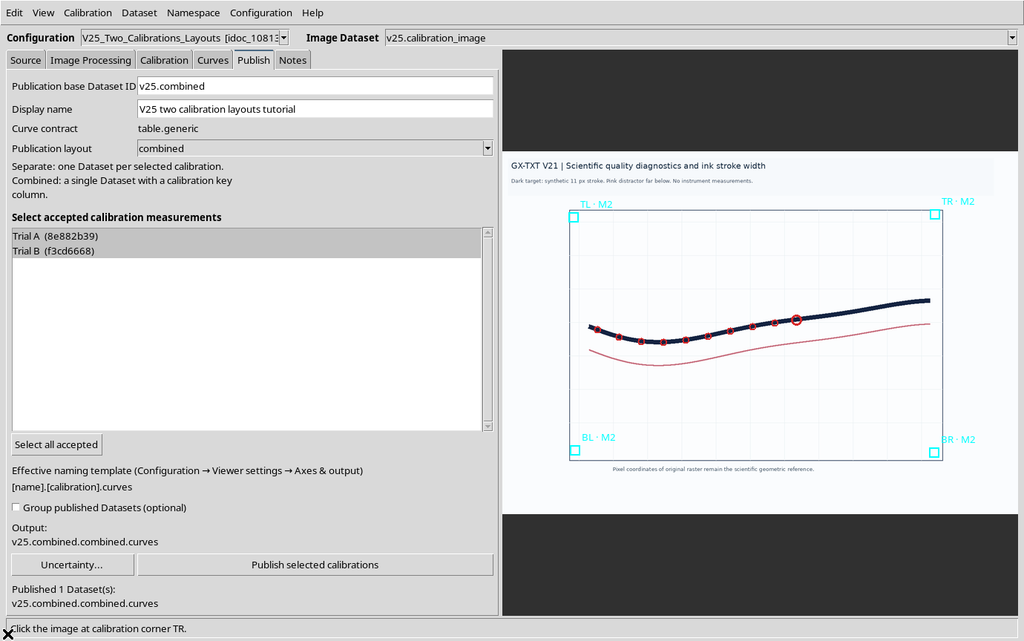
The original data are not repeated to simulate an experimental replicate: they are the coordinates transformed by the two selected calibration models.
31. Combined Requires a Calibration Key per Row
The Combined Dataset contains a column referring to the calibration, in addition to the scientific coordinates. This makes it possible to separate the results of Trial A and Trial B even when they are stored in the same object.
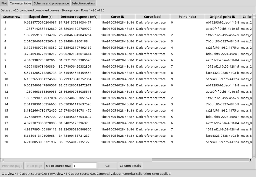
When the data are exported or processed, the calibration key must not be lost. A comparison that ignores its presence can mix values obtained with different transformations.
32. The Numerical Schema Describes the Roles of the Variables
The CORE schema view exposes the columns and roles actually published. The Combined case includes the identities of the curve and of the calibration, in addition to X, Y and the references of the original points.
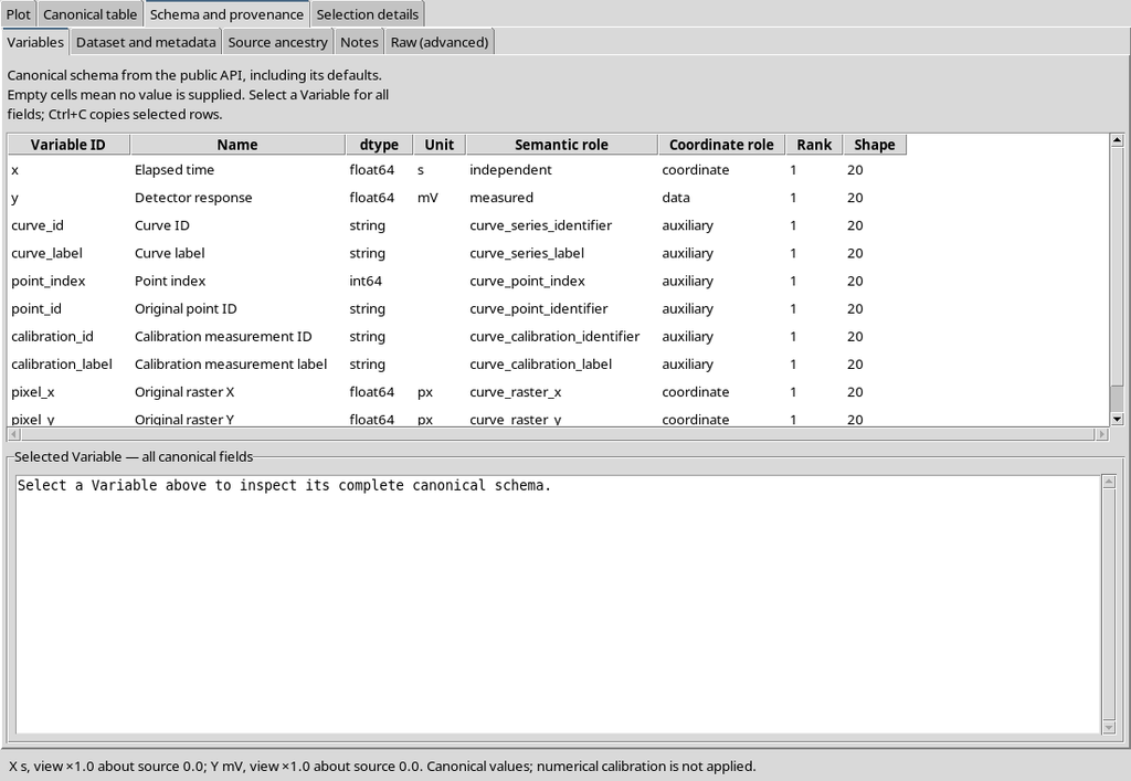
The schema is more reliable than the visual order of the columns for recognizing curve_key, calibration_key, scientific coordinates and references to the raster.
33. Comparison of the Two Layouts
| Criterion | Separate | Combined |
|---|---|---|
| Realizations selected in the example | Trial A + Trial B | Trial A + Trial B |
| Resulting numerical Datasets | 2 | 1 |
| Total rows | 10 + 10 | 20 |
| Calibration association | Identity of the individual output and its metadata | Calibration key per row |
| Starting source | The same ten raster points | The same ten raster points |
| Scientific result | Two transformations kept separate | Two transformations gathered in one table |
The total number of transformed points is the same in the two layouts. These are not two different measurement algorithms: the main difference is the structure through which the realizations are made available.
34. Y1 and Y2 with the Same Physical Unit
A different comparison concerns two logical Y axes. When Y1 and Y2 are associated with the same physical unit — for example both in mV — a Combined output can contain the two series in the same table, distinguishing them through the axis identifier.
Do not confuse Combined for calibrations with Y1/Y2: they are two independent dimensions of publishing. A specific configuration can use them at the same time.
35. The Mixed Publication with Equal Units Keeps 19 Rows
In the case with eight points on Y1 and eleven on Y2, both in mV, the Viewer produced a 19-row Dataset. The Y1/Y2 distinction remains represented in the canonical data.
A single Dataset does not mean that every point uses the same logical axis: the published y_axis_id role must be consulted.
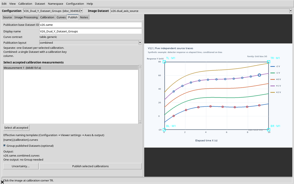
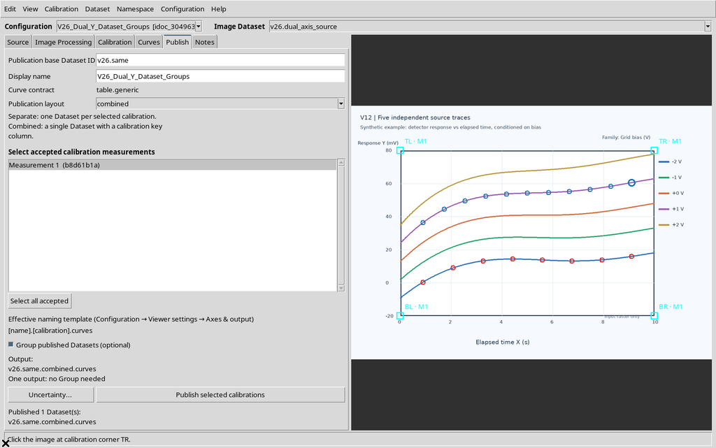
36. A Single Output Does Not Require a Dataset Group
The Group published Datasets option serves to associate several Datasets, when there really are several outputs to group. If the publication produces a single numerical Dataset, the system may indicate that no Group is needed.
The ticked box does not guarantee that a group will be created. Before looking for a Group object in the browser, check the actual number of numerical outputs generated.
37. Two Different Y Units Require Consistent Separation
When Y1 is expressed in mV and Y2 in deg, the situation is different. The system must not indiscriminately merge amplitude and phase values into a single Y column without physical distinction.
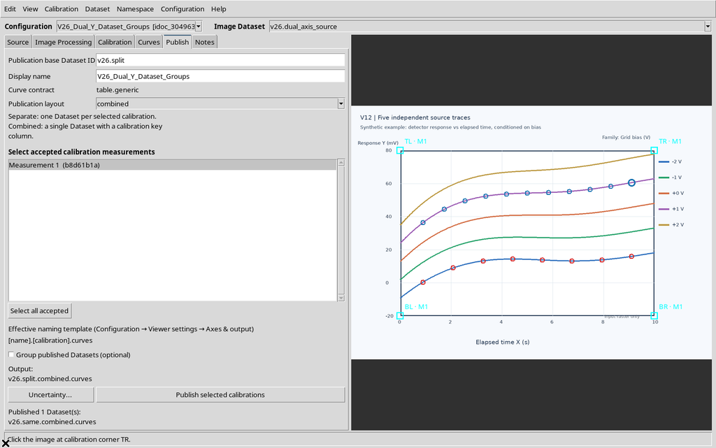
The word Combined in the plan concerns the structure of the realizations, not an authorization to confuse two physical quantities.
38. Two Datasets for Y1 and Y2 with Different Units
In the case observed, after Publish, two numerical Datasets were produced: the Y1 member with 8 rows in mV and the Y2 member with 11 rows in deg.
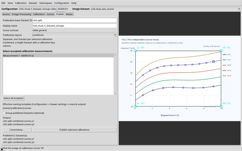
Even though the outputs derive from the same image and the same calibration geometry, they represent distinct physical variables. Keeping the unit of each member is an essential requirement.
39. The Dataset Group Links the Outputs Without Merging Them
If the user enables Group published Datasets in a situation with several compatible results, the framework can create a Group that associates them. In the case observed the two Y1 and Y2 Datasets were registered, plus a Group.
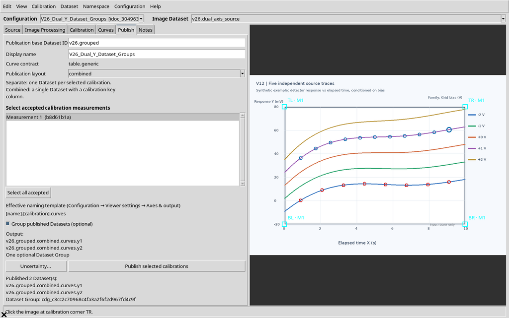
The Group does not create new scientific rows. The two members remain separate Datasets, with their original contents and units.
40. Inspecting the Group Members in the CORE
In the framework browser a Group can appear as a node with associated members. The Inspect Group command lets you consult the roles, status and digital fingerprints of the outputs.
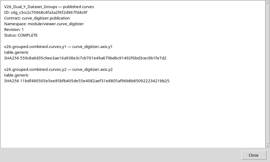
The example shows a Group status of COMPLETE, with separate roles for Y1 and Y2. Do not confuse the Group node with a third numerical Dataset.
41. An Ordinary Plot Can Show a Mixed Dataset with Common Units
The standard CORE scientific Viewer lets you consult the Y1/Y2 Dataset with equal units. In this case the mixed publication contains 19 rows, with the logical axis association stored in the Dataset.
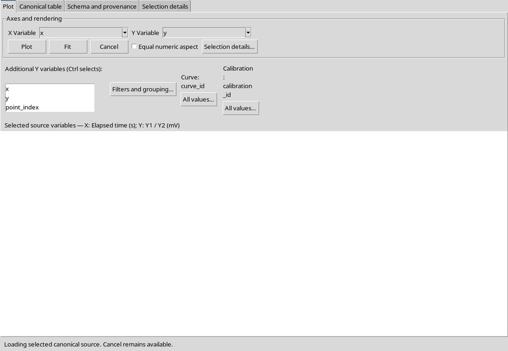
The presence of a standard CORE plot is not enough to prove that the additional Curves tab with a native dual axis in Plot v4 has also been exercised.
42. The Y1 Dataset in mV Can Be Consulted Separately
After separation by physical unit, the Y1 member can be displayed on its own. In the documented case it contains eight points and keeps the vertical axis in millivolts.
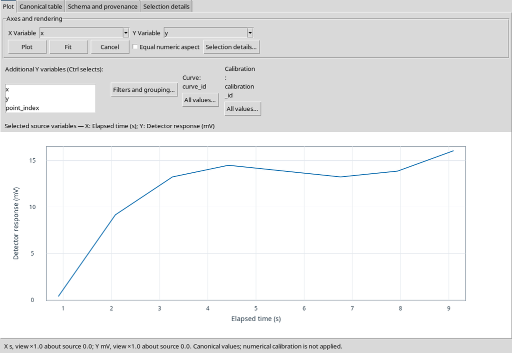
This output is a canonical Dataset actually published, not an image cropped from the dual-axis plot.
43. The Y2 Dataset in Degrees Keeps Another Quantity
The Y2 member contains eleven points, with the ordinate in degrees. Its representation is distinct from the Y1 one and requires a reading consistent with the physical unit of phase.
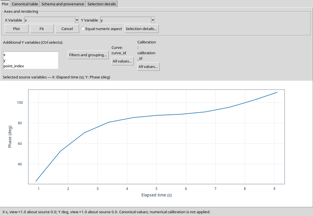
Using the same original raster does not automatically turn the phase into an amplitude. The axis labels and metadata must accompany each output.
44. The Limits of the Views Illustrated
This guide illustrates the configuration of the secondary axis, the verification of X/Y1/Y2 coordinates, the publication of Datasets with equal or different units, the CORE scientific Viewer plots and the structure of Dataset Groups. These features must be kept distinct from the representation in the Curves contribution with two physically different Y axes.
Similarly, the Canonical Data example presented here concerns a Dataset published in Separate mode with one calibration. The Combined Dataset with several realizations, instead, is illustrated in the ordinary CORE scientific Viewer. To use a different combination of views and publications, check the rows and calibration keys of your own Dataset directly.
45. Plot v4 on the Separate Dataset Remains Valid
In an example with three synthetic curves and 66 points, the additional Curves tab displays the series with Plot Dataset API v4. This is a Separate publication with a single Y axis.
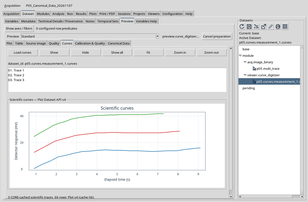
The same numerical origin is available in Canonical Data, but the arrangement of the values is different from the plot.
46. Hiding a Line in Plot v4 Does Not Delete Its Points
In the comparison the Hide and Show all actions were applied. Hide removes one of the three lines from the presentation, without acting on the registered scientific rows.
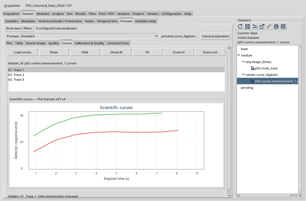
The change of representation is not an operation of cleaning data or discarding unwanted points.
47. Canonical Data Continues to Show All the Rows
Reopening Canonical Data after the visibility change, the table keeps the values of the hidden curve. Reading both pages confirmed the identity of all 66 published rows.
This is one of the most useful checks to carry out when working with several views: changing what is visible must not rewrite what has been published.
To verify the persistence of the data after Hide or Show all, return to Canonical Data and select the same Point traceability page. The table must still contain the points of the hidden curve, together with the identifiers and the original raster coordinates.
The traceability screen coincides with the one already illustrated in section 17: there is no need to duplicate it. The correct comparison concerns Dataset ID, Point ID, number of rows and numerical values; the temporary presence or absence of a line in the Plot is not a scientific modification.
48. Comparison Matrix of the Observed Conditions
| Comparison | Documented result | Scope |
|---|---|---|
| Empty Session / Image Dataset | No numerical data / original raster viewable | Ordinary Preview |
| Raster / curve Dataset | Original pixels / numerical rows with axes and provenance | Ordinary Preview and canonical Dataset |
| Standard Plot / additional Curves | Different views of published data; Curves offers a dedicated list and commands | Single Y axis verified |
| Standard Quality / Calibration & Quality | Diagnostics table / summary of calibration metadata | One compatible numerical Dataset |
| Scientific values / Point traceability | Physical coordinates / IDs and original pixel coordinates | Two views of the same rows |
| Separate / Combined | Two 10-row Datasets / one 20-row Dataset | Two accepted realizations |
| Y1/Y2 in the same unit | One mixed 19-row Dataset | Two logical axes, mV |
| Y1/Y2 in different units | Two Datasets with 8 and 11 rows | Y1 mV, Y2 deg |
| Two outputs with Group | Two Datasets and an associative Group | Declared roles and integrity |
| Precision 6/10/Full | Changes the displayed numerical text, not the values | Canonical Data |
| Hide/Show all | Changes the presence of lines in the Plot, not the canonical rows | Curves, Plot Dataset API v4 |
The matrix gathers distinct teaching examples and highlights their conditions of use. Differences in the number of points and in the calibrations do not constitute physical results comparable with each other.
49. When Checks on Other Data Combinations Are Needed
If you want to use Curves with two physically different Y quantities, you need to check the behaviour of the plot directly on your own publication. Likewise, with a Combined Dataset containing several calibrations, check in Canonical Data that the respective keys are available and recognizable.
For a Bode-type plot, with logarithmic X and different Y1/Y2 axes, consistent checks are needed on source, calibration, points, publication, plot and table. The functioning of a specific display must not be inferred merely from the fact that another CORE tab correctly shows the same data.
50. Checklist for Choosing a Reliable View
Before interpreting a figure, check: which Session is open, which Dataset is selected, which contract is published, how many points and calibrations it contains, which physical units are declared and whether the operation performed concerns data or only the display.
In a publication with several realizations, keep the calibration keys; for Y1/Y2 do not mix incompatible units; in the presence of a Dataset Group check the individual members; in Calibration & Quality distinguish software checks from metrological accuracy. For scientific processing always use the values of the canonical Dataset and its provenance, not just the pixels shown on the screen.