

OpenFOAM: CFD capstone project of a porous-bed reactor
Twentieth and last guide of the Learning OpenFOAM 14 path and the fourth of the “Advanced transport and final project” module of the advanced course, after those on server and transfers, monitoring and convergence, quantitative analysis with ParaView, verification and validation, parameter sweeps, mesh generation, boundary conditions and models, transient simulations, turbulence and RANS models, heat transfer, conjugate heat transfer, species transport, VOF multiphase flows, porous media, rotating machinery, dynamic meshes, dispersed particles, chemical reactions and numerical methods and performance. This is the capstone project: a channel reactor with a homogenised porous insert, from the research question to the scientific report, with a 12-case campaign, pressure and flow-rate measurements, balances, a mesh study and a PFR kinetic estimate kept separate from the CFD. The deep-dive and practical-tip boxes open with a click: they contain every script and file of the package, the OpenFOAM 14 code of the Darcy–Forchheimer term, the numbers of the case (Re 25–100, a 0.1 mm Brinkman layer, expected ΔP 68.5 Pa against 60 from the Darcy formula), the exact solution of the developed stretch and what each mesh returns of it, the equivalence with a bed of spheres according to Ergun, the Thiele, Weisz–Prater and Mears criteria, nine additional tested scripts (a-priori estimates, exact solution, measurements written by the solver on generated planes, extraction with evidence, regressions, mesh series and GCI, runs with verified status, the reaction solved by OpenFOAM 14 in the bed) and linked bibliographic references. The archive with all scripts and files is available for download at the end of the article.
Practical OpenFOAM series · From geometry to a scientific report
Reference environment: OpenFOAM Foundation 14 running on Linux; Windows with FileZilla, Notepad++ and ParaView 5.13.2 connected to pvserver.
Level: advanced capstone. Final deliverable: an auditable collection of cases, logs, plots, measurements, checks and a scientific report.
Scientific scope. The supplied CFD case solves incompressible fluid flow with an additional hydraulic resistance representing the porous insert. Chemical conversion is evaluated separately using an analytical plug-flow reactor (PFR) model: it is NOT computed by the OpenFOAM solver. This distinction must be retained in the final report.
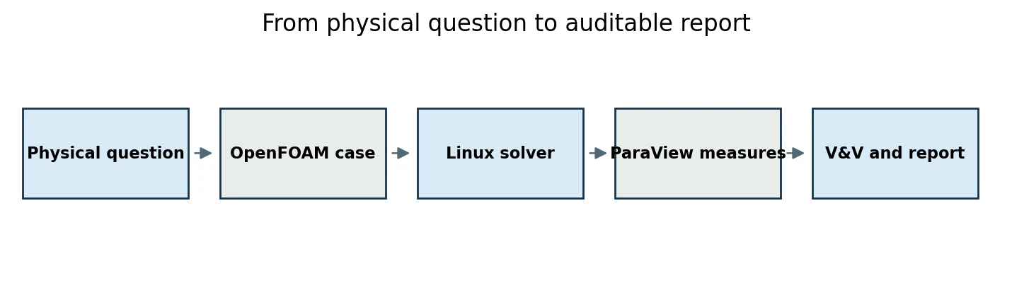
1. The research question
A liquid flows through a small rectangular channel containing a central region that represents a homogenized porous catalyst support. We ask how the pressure loss and nominal residence time change with the inlet flow rate and the resistance of the porous section, and how a preliminary first-order reaction estimate may enter an engineering trade-off.
Direct CFD observables: kinematic pressure, velocity field, volume flow rate and continuity balance. Derived observables: pressure loss in pascals, hydraulic resistance and, under additional stated assumptions, a nominal residence time and ideal conversion. Neither microscopic catalyst geometry nor coupled reacting-flow physics is claimed.
Deep dive · The case in numbers: Reynolds numbers, gradients, Brinkman layer, time scales and conversion
Before launching the first run it pays to know what to expect. extra/case_estimates.py reads the dictionaries of a prepared case (blockMeshDict, createZonesDict, 0/U, physicalProperties, fvModels, controlDict), counts the cells whose centre falls inside the reactorBed box (the same criterion as createZones) and computes the quantities that govern the physics and the numerics of the problem. For the central case (U = 0.015 m/s, d = 10⁸ m⁻²):
| Quantity | Value | Consequence |
|---|---|---|
| porous-zone cells | 2560 (32 × 20 × 4), from 40 to 80 mm, volume 8.0·10⁻⁷ m³ | the planes x = 35, 40, 80, 85 mm lie on cell faces also for the 48×10×2 and 192×40×8 meshes: the zone volume is exact |
| hydraulic diameter Dh = 4A/P | 3.333 mm | ReDh = U·Dh/ν = 25, 50, 100: laminar flow in the whole campaign |
| permeability Reynolds number ReK = U√K/ν | 0.75 – 1.5 – 3 (d = 10⁸) | at the upper limit of the Darcy regime: for a real medium the Forchheimer term is no longer negligible (section 5) |
| entrance length (Durst et al. 2005) | 5.5 – 10 – 19 mm | the 35 mm plane sees a developed profile; the 85 mm plane is 5 mm after the bed, in the re-development zone |
| Darcy-only ΔP μ·d·L·U (guide formula) | 60 Pa | the volumetric resistance of the insert alone |
| developed gradient in the bed, exact solution | 1700 Pa/m = 1.133 × Darcy | wall friction inside the bed (Brinkman layer) adds 13 % |
| expected ΔP between 35 and 85 mm (developed, exact) | 68.5 Pa (= 0.0685 m²/s² of kinematic p) | mesh-independent reference value; without the insert the same stretch gives 2.6 Pa |
| Brinkman length √K = 1/√d | 0.10 mm = 0.2 of the cell side (0.5 mm) | the boundary layer inside the bed is not resolved by the base mesh (sections 8 and 17) |
| time scales | viscous 0.39 s; Darcy relaxation 1/(νd) = 0.01 s; flow-through L/U = 16 – 8 – 4 s | the velocity field settles in a few seconds; a transported scalar instead needs several flow-through times (section 10) |
| time step | 0.01 s, limited by maxDeltaT (maximum Courant number 0.10 – 0.21 – 0.41) | about 1600 steps to 16 s for every case of the campaign |
| analytical PFR (not CFD) | τ = 1.867 s, X = 8.911 % | matches the value of section 14 |
Run on the central case prepared with prepare_campaign.py:
$ python3 extra/case_estimates.py run01/U0.0150_D1e08
Case run01/U0.0150_D1e08
  domain 120 x 10 x 2 mm, mesh 96 x 20 x 4 = 7680 cells, cell 1.25 x 0.5 x 0.5 mm (aspect ratio 2.5)
  reactorBed: 2560 cells with centre in the box, x = 40-80 mm, volume 8e-07 m3 (guide: 8.0e-07)
  inlet U = 0.015 m/s, A = 2e-05 m2, Q = 3e-07 m3/s; Dh = 3.333 mm, Re_Dh = 50.0 (laminar)
  entrance length about 10.0 mm: the 35 mm section is developed; 85 mm is 5 mm after the bed, inside the re-development zone
  d = 1e+08 1/m2: K = 1e-08 m2, sqrt(K) = 0.1000 mm = 0.20 of the smallest cell side; Re_K = U sqrt(K)/nu = 1.50
  Darcy only (guide formula) mu d L U = 60 Pa
  fully developed (exact): duct 51.49 Pa/m, bed 1699.6 Pa/m (x1.1331 of Darcy)
  expected dP between x = 35 and 85 mm: about 68.5 Pa (= 0.0685 m2/s2 of kinematic p); whole duct without bed 6.18 Pa
  time scales: viscous decay 0.39 s, Darcy relaxation 0.01 s, flow-through L/U 8 s
  time step 0.01 s (maxCo 0.5, maxDeltaT 0.01) -> about 1600 steps to endTime 16 s
  analytical PFR (NOT CFD): eps 0.7, k 0.05 1/s -> tau = 1.867 s, X = 8.911 %
[exit 0]
With several cases the script prints one line per case: it is the table of expected values of the campaign (section 9). The complete code is in the section 3 box.
Practical tip · The project tools: which script, when, what it produces
| Script | When | What it produces |
|---|---|---|
exercises/prepare_campaign.py | first | 12 cases (or 3 with --quick) and manifest.csv (section 9) |
extra/case_estimates.py | before the run | expected numbers of the case or campaign (sections 1 and 3) |
extra/fully_developed.py | before the run | exact and on-mesh gradients, expected ΔP between the planes, PFR and segregated conversion (section 13) |
extra/bed_equivalence.py | at design stage | equivalent bed of spheres, neglected Forchheimer term, Damköhler, dispersion, Thiele (sections 5 and 14) |
extra/add_monitors.py | on never-run cases | pressures on the planes, flow rates, profiles and residuals written by the solver (section 11) |
extra/add_reaction_tracer.py | optional, on never-run cases | first-order reaction solved by OpenFOAM in the bed (section 20) |
exercises/run_case.sh or extra/run_case_checked.sh | one run per case | four logs; the checked version adds input hashes and RUN_SUCCESS/RUN_FAILED status (section 8) |
extra/extract_measurements.py | after the runs | the measurements CSV in the package format and the evidence file (section 12) |
exercises/analyze_measurements.py | after extraction | ΔP in Pa, Darcy estimate, balance, analytical τ and X (section 18) |
extra/campaign_fit.py | Exercise B | ΔP(U) regressions, insert contribution, apparent permeability (section 16) |
extra/prepare_mesh_series.py, extra/gci.py | Exercise C | three meshes and GCI index (section 17) |
exercises/snapshot_inputs.py | before and after every run | SHA-256 hashes of the inputs (section 18) |
All scripts are in the archive at the end of the article: exercises/ is the guide package (with template/), extra/ the additional scripts presented in the boxes. They use only the Python 3 standard library, except the optional plot of campaign_fit.py (matplotlib).
2. Objectives and prerequisites
By completing the capstone, a reader should be able to frame a testable question, design a new CFD case using traceable syntax, automate a parameter sweep without destroying previous work, measure physical observables rather than merely collecting colorful figures, perform basic verification and produce a reproducible scientific report.
This guide integrates the skills of Guides 1–19: Windows/Linux operation, dictionaries, mesh generation, foamRun, log inspection, ParaView, fvModels, convergence analysis and numerical sensitivity. No Visual Studio Code is required.
Deep dive · Code verification, solution verification, validation: what this project can demonstrate
The literature on CFD credibility distinguishes three activities (Oberkampf and Trucano 2002, doi:10.1016/S0376-0421(02)00005-2; Roache 1997, doi:10.1146/annurev.fluid.29.1.123):
- code verification: the program correctly solves the equations it claims to solve. Here an exact reference exists: in the developed parts of the channel and the bed the 3D problem reduces to a cross-section equation with a series solution (section 13). Comparing the measured pressure gradient with the one computed on the same grid by
fully_developed.pychecks the whole chain (mesh, zone, porous model, boundary conditions); - solution verification: estimating the numerical error of a result (iterative, temporal, discretisation error), with the GCI of Exercise C (Roache 1994, doi:10.1115/1.2910291; Celik et al. 2008, doi:10.1115/1.2960953);
- validation: the model represents the real device. It requires independent measurements (ΔP–Q of a real bed, measured conversion) that this project does not have: the conclusions must stay within verification.
A falsifiable question, stated before the runs, can be: “in the 35–85 mm stretch the insert contribution ΔP(d) − ΔP(0) is proportional to U within 1 % and equals μdLU times a wall factor between 1 and 1.2”. The exact prediction (section 13) gives 1.099 for d = 10⁸; the base mesh returns about 1.016: the comparison tells how much the wall resolution weighs on the observable.
Practical tip · Where to review each required skill
| Project step | Reference guide |
|---|---|
| Linux server, FileZilla, Notepad++, pvserver | Guide 1, Guide 3 |
| logs, residuals, continuity, Courant number | Guide 2, Guide 8 |
| GCI and mesh independence | Guide 4 |
| campaigns without overwriting | Guide 5 |
blockMesh, checkMesh, zones | Guide 6 |
| boundary conditions | Guide 7 |
| porosityForce and Darcy–Forchheimer | Guide 14 |
| species transport, reactions | Guide 12, Guide 18 |
| schemes, solvers, performance | Guide 19 |
3. Physical geometry and dimensions
The rectangular duct has length 120 mm, width 10 mm and height 2 mm. The porous portion extends from x = 40 mm to x = 80 mm and covers the whole cross-section. The baseline mesh has 96 × 20 × 4 = 7,680 cells. The porous region is the reactorBed cellZone, not a geometrically resolved solid.
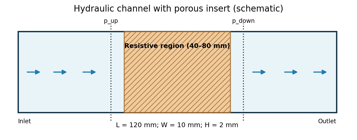
| Quantity | Demonstration value | Interpretation |
|---|---|---|
| Cross-sectional area A | 2.0 × 10⁻⁵ m² | Q = A · Uᵢₙ for uniform inlet velocity |
| Bed geometric volume V | 8.0 × 10⁻⁷ m³ | A × 0.04 m |
| Kinematic viscosity ν | 1.0 × 10⁻⁶ m²/s | Fluid model input |
| Density ρ | 1,000 kg/m³ | Assumed only for pressure conversion and dynamic viscosity |
| Darcy coefficient d | 0, 5×10⁷, 10⁸, 2×10⁸ m⁻² | Controls porous resistance |
| Inlet speed Uᵢₙ | 0.0075, 0.015, 0.03 m/s | Sets the imposed flow rate |
These are teaching assumptions, not measurements from a physical device. Actual geometric and material parameters must be documented with sources and uncertainty estimates before extrapolation.
Deep dive · The case_estimates.py code
The script reads the numbers directly from the dictionaries, so it also works for modified copies (refined meshes, different velocities or resistances). The developed gradient comes from fully_developed.py (same folder, section 13); the entrance length uses the Durst et al. correlation (2005, doi:10.1115/1.2063088) with Dh; the Courant number is computed along x with the maximum velocity of the developed profile (1.715 U, from the exact series).
#!/usr/bin/env python3
# SPDX-License-Identifier: GPL-3.0-or-later
"""A-priori numbers of a Guide 20 reactor case, read from its dictionaries.

Reads system/blockMeshDict (vertices, nx ny nz), system/createZonesDict (box),
0/U (inlet velocity), constant/physicalProperties (nu), constant/fvModels
(D, f) and system/controlDict (endTime, deltaT, maxCo, maxDeltaT) and prints:

  * mesh: cells, cell sizes, aspect ratio; cells whose centre is inside the
    reactorBed box (what createZones selects), their x range and volume;
  * flow: section, flow rate, hydraulic diameter, Reynolds numbers (duct and
    permeability based), entrance length (Durst et al. 2005);
  * pressure: Darcy-only estimate mu*d*L*U, fully developed duct and bed
    gradients (exact series of fully_developed.py, same folder), expected
    pressure drop between the 35 and 85 mm sections;
  * Brinkman length sqrt(1/d) compared with the cell height;
  * time scales: viscous decay, Darcy relaxation 1/(nu*d), flow-through
    time, time step allowed by maxCo and maxDeltaT, number of steps;
  * the analytical PFR estimate of the guide (void fraction 0.70, k 0.05 1/s).

Nothing is written. Several cases give one summary line each.

Usage: python3 case_estimates.py CASE [CASE ...] [--rho 1000] [--void-fraction 0.7] [--k 0.05]
"""
import argparse, math, os, re, sys
sys.path.insert(0, os.path.dirname(os.path.abspath(__file__)))
import fully_developed as FD


def text(case, rel):
    t = open(os.path.join(case, rel), encoding='utf-8').read()
    return re.sub(r'//.*', '', re.sub(r'/\*.*?\*/', '', t, flags=re.S))


def scalar(t, key, default=None):
    m = re.search(r'(?m)^\s*' + re.escape(key) + r'\s+([-+0-9.eE]+)\s*;', t)
    if m:
        return float(m.group(1))
    if default is None:
        raise KeyError(key)
    return default


def vec(s):
    return [float(v) for v in s.split()]


def read_case(case):
    bm = text(case, 'system/blockMeshDict')
    n = [int(scalar(bm, k)) for k in ('nx', 'ny', 'nz')]
    verts = [vec(v) for v in re.findall(r'\(\s*([-+0-9.eE]+\s+[-+0-9.eE]+\s+[-+0-9.eE]+)\s*\)',
                                         re.search(r'vertices\s*\((.*?)\n\s*\);', bm, re.S).group(1))]
    lo = [min(v[i] for v in verts) for i in range(3)]
    hi = [max(v[i] for v in verts) for i in range(3)]
    cz = text(case, 'system/createZonesDict')
    b = re.search(r'box\s*\(([^)]*)\)\s*\(([^)]*)\)', cz)
    box = (vec(b.group(1)), vec(b.group(2)))
    u = text(case, '0/U')
    inlet = re.search(r'inlet\s*\{[^}]*value\s+uniform\s*\(([^)]*)\)', u, re.S)
    U = vec(inlet.group(1))[0]
    nu = scalar(text(case, 'constant/physicalProperties'), 'nu')
    fv = text(case, 'constant/fvModels')
    D = scalar(fv, 'D')
    fm = re.search(r'(?m)^\s*f\s*\(([^)]*)\)', fv)
    f = vec(fm.group(1))[0] if fm else 0.0
    cd = text(case, 'system/controlDict')
    ctl = {k: scalar(cd, k, float('nan')) for k in ('endTime', 'deltaT', 'maxCo', 'maxDeltaT')}
    return dict(n=n, lo=lo, hi=hi, box=box, U=U, nu=nu, d=D, f=f, **ctl)


def estimates(c, rho, eps, k):
    (nx, ny, nz), lo, hi = c['n'], c['lo'], c['hi']
    L, W, H = (hi[i] - lo[i] for i in range(3))
    dx, dy, dz = L / nx, W / ny, H / nz
    bl, bh = c['box']
    sel = [i for i in range(nx) if bl[0] <= lo[0] + (i + 0.5) * dx <= bh[0]]
    full = all(bl[j] <= lo[j] + 0.5 * h and bh[j] >= hi[j] - 0.5 * h for j, h in ((1, dy), (2, dz)))
    ncz = len(sel) * (ny * nz if full else 0)
    x0, x1 = lo[0] + sel[0] * dx, lo[0] + (sel[-1] + 1) * dx
    Vz = ncz * dx * dy * dz
    A = W * H
    U, nu, d = c['U'], c['nu'], c['d']
    mu = rho * nu
    Q = A * U
    Dh = 4 * A / (2 * (W + H))
    Re = U * Dh / nu
    Le = Dh * (0.619 ** 1.6 + (0.0567 * Re) ** 1.6) ** (1 / 1.6)
    FD.W, FD.H = W, H
    g_duct = mu * U / FD.exact_mean(0.0)
    g_bed = mu * U / FD.exact_mean(d) if d > 0 else g_duct
    Lb = x1 - x0
    dp_darcy = mu * d * Lb * U
    dp_35_85 = g_duct * (0.05 - Lb) + g_bed * Lb
    t_visc = 1 / (nu * math.pi ** 2 * (1 / W ** 2 + 1 / H ** 2))
    umax = 1.715 * U        # centre-line velocity of the developed 10 x 2 mm duct profile (exact series)
    dt = min(c['maxDeltaT'], c['maxCo'] * dx / umax)     # flow along x: Co = u dt / dx
    tau = eps * Vz / Q
    return dict(L=L, W=W, H=H, dx=dx, dy=dy, dz=dz, cells=nx * ny * nz, ncz=ncz, x0=x0, x1=x1, Vz=Vz, A=A, Q=Q, Dh=Dh, Re=Re,
                ReK=(U / math.sqrt(d) / nu if d > 0 else float('nan')), Le=Le, g_duct=g_duct, g_bed=g_bed, dp_darcy=dp_darcy,
                dp_35_85=dp_35_85, sqrtK=(1 / math.sqrt(d) if d > 0 else float('inf')), t_visc=t_visc,
                t_darcy=(1 / (nu * d) if d > 0 else float('inf')), t_flow=L / U, dt=dt, steps=c['endTime'] / dt,
                tau=tau, X=1 - math.exp(-k * tau), forch=(c['f'] * U / (2 * nu * d) if d > 0 else 0.0))


def report(case, c, e, rho, eps, k):
    p = print
    p(f'Case {case}')
    p(f'  domain {e["L"]*1e3:g} x {e["W"]*1e3:g} x {e["H"]*1e3:g} mm, mesh {c["n"][0]} x {c["n"][1]} x {c["n"][2]} = {e["cells"]} cells, '
      f'cell {e["dx"]*1e3:g} x {e["dy"]*1e3:g} x {e["dz"]*1e3:g} mm (aspect ratio {max(e["dx"], e["dy"], e["dz"])/min(e["dx"], e["dy"], e["dz"]):g})')
    p(f'  reactorBed: {e["ncz"]} cells with centre in the box, x = {e["x0"]*1e3:g}-{e["x1"]*1e3:g} mm, volume {e["Vz"]:.4g} m3 (guide: 8.0e-07)')
    p(f'  inlet U = {c["U"]:g} m/s, A = {e["A"]:.3g} m2, Q = {e["Q"]:.4g} m3/s; Dh = {e["Dh"]*1e3:.3f} mm, Re_Dh = {e["Re"]:.1f} (laminar)')
    p(f'  entrance length about {e["Le"]*1e3:.1f} mm: the 35 mm section is developed; 85 mm is {(0.085-e["x1"])*1e3:g} mm after the bed, inside the re-development zone')
    if c['d'] > 0:
        p(f'  d = {c["d"]:.4g} 1/m2: K = {1/c["d"]:.3g} m2, sqrt(K) = {e["sqrtK"]*1e3:.4f} mm = {e["sqrtK"]/min(e["dy"], e["dz"]):.2f} of the smallest cell side; '
          f'Re_K = U sqrt(K)/nu = {e["ReK"]:.2f}')
    else:
        p('  d = 0: control case, the zone exists but adds no force')
    if c['f']:
        p(f'  f = {c["f"]:g} 1/m: Forchheimer/Darcy ratio f U/(2 nu d) = {e["forch"]:.3g}')
    p(f'  Darcy only (guide formula) mu d L U = {e["dp_darcy"]:.4g} Pa')
    p(f'  fully developed (exact): duct {e["g_duct"]:.4g} Pa/m, bed {e["g_bed"]:.5g} Pa/m '
      f'(x{e["g_bed"]/max(rho*c["nu"]*c["d"]*c["U"], 1e-300):.4f} of Darcy)' if c['d'] > 0 else
      f'  fully developed (exact): duct {e["g_duct"]:.4g} Pa/m')
    p(f'  expected dP between x = 35 and 85 mm: about {e["dp_35_85"]:.4g} Pa (= {e["dp_35_85"]/rho:.4g} m2/s2 of kinematic p); '
      f'whole duct without bed {e["g_duct"]*e["L"]:.3g} Pa')
    p(f'  time scales: viscous decay {e["t_visc"]:.3g} s, Darcy relaxation {e["t_darcy"]:.3g} s, flow-through L/U {e["t_flow"]:.3g} s')
    p(f'  time step {e["dt"]:.3g} s (maxCo {c["maxCo"]:g}, maxDeltaT {c["maxDeltaT"]:g}) -> about {e["steps"]:.0f} steps to endTime {c["endTime"]:g} s')
    p(f'  analytical PFR (NOT CFD): eps {eps:g}, k {k:g} 1/s -> tau = {e["tau"]:.4g} s, X = {100*e["X"]:.3f} %')


def main():
    ap = argparse.ArgumentParser(description=__doc__.split('\n')[0])
    ap.add_argument('cases', nargs='+')
    ap.add_argument('--rho', type=float, default=1000.0)
    ap.add_argument('--void-fraction', type=float, default=0.7)
    ap.add_argument('--k', type=float, default=0.05)
    a = ap.parse_args()
    res = []
    for case in a.cases:
        if not os.path.isdir(case):
            continue
        try:
            c = read_case(case)
        except (OSError, KeyError, AttributeError) as ex:
            print(f'{case}: cannot read the dictionaries ({ex})')
            continue
        e = estimates(c, a.rho, a.void_fraction, a.k)
        res.append((case, c, e))
    if len(res) == 1:
        report(*res[0], a.rho, a.void_fraction, a.k)
        return
    print(f'{"case":28s} {"cells":>6s} {"U m/s":>7s} {"d 1/m2":>8s} {"Re":>6s} {"Darcy Pa":>9s} {"dP35-85 Pa":>10s} {"steps":>6s} {"tau s":>6s} {"X %":>6s}')
    for case, c, e in res:
        print(f'{os.path.basename(os.path.normpath(case)):28s} {e["cells"]:6d} {c["U"]:7.4f} {c["d"]:8.2g} {e["Re"]:6.1f} '
              f'{e["dp_darcy"]:9.3f} {e["dp_35_85"]:10.3f} {e["steps"]:6.0f} {e["tau"]:6.3f} {100*e["X"]:6.2f}')


if __name__ == '__main__':
    main()
Practical tip · The domain and the zone in the case files
The geometry is entirely in system/blockMeshDict (a single block, macros nx ny nz), the zone in system/createZonesDict: the box extends beyond the walls in y and z (from −1 to 11 mm and from −1 to 3 mm) to include all the cell centres of the section with certainty. The criterion is the cell centre: with spacings that do not divide 40 and 80 mm exactly the zone would have a volume different from A·0.04 m³, and the estimate τ = εV/Q would have to be corrected with the actual volume (section 8 box).
system/blockMeshDict
/* Guide 20: idealised channel reactor mesh; dimensions in SI units. */
FoamFile
{
    version 2.0;
    format ascii;
    class dictionary;
    object blockMeshDict;
}

nx 96;
ny 20;
nz 4;

vertices
(
    (0 0 0)
    (0.12 0 0)
    (0.12 0.01 0)
    (0 0.01 0)
    (0 0 0.002)
    (0.12 0 0.002)
    (0.12 0.01 0.002)
    (0 0.01 0.002)
);

blocks
(
    hex (0 1 2 3 4 5 6 7) ($nx $ny $nz) simpleGrading (1 1 1)
);

edges ();

boundary
(
    inlet
    {
        type patch;
        faces ((0 4 7 3));
    }
    outlet
    {
        type patch;
        faces ((1 2 6 5));
    }
    walls
    {
        type wall;
        faces
        (
            (0 1 5 4)
            (3 7 6 2)
            (0 3 2 1)
            (4 5 6 7)
        );
    }
);
mergePatchPairs ();
system/createZonesDict
/* Define a cell zone spanning the complete channel cross-section. */
FoamFile
{
    version 2.0;
    format ascii;
    class dictionary;
    object createZonesDict;
}
reactorBed
{
    type box;
    zoneType cell;
    box (0.04 -0.001 -0.001) (0.08 0.011 0.003);
}
constant/physicalProperties
FoamFile
{
    version 2.0;
    format ascii;
    class dictionary;
    location "constant";
    object physicalProperties;
}
viscosityModel constant;
nu 1e-06;
constant/momentumTransport
FoamFile
{
    version 2.0;
    format ascii;
    class dictionary;
    location "constant";
    object momentumTransport;
}
simulationType laminar;
ρ = 1000 kg/m³ appears in no file: the incompressible solver works with p/ρ and ν. ρ only enters the conversion to pascal and μ = ρν in the analytical formulas; use the same value in every processing step (option --rho of the scripts).
4. Equations actually solved in CFD
OpenFOAM solves the incompressible continuity and momentum equations in the fluid volume and applies an additional resistance term within the selected porous cells. For a Darcy–Forchheimer material, the physical resistance term is:
The coefficient d has units m⁻², while f has units m⁻¹. This experiment deliberately sets f = 0, isolating the linear Darcy resistance. A later nonzero Forchheimer term would require a separate velocity-scaling study.
The porosityForce model is defined in constant/fvModels; system/createZonesDict selects cells between 40 and 80 mm. constant/coordinateSystems establishes the reference axes; equal d coefficients along the three axes represent isotropic resistance.
Optional reminder — kinematic pressure. In this incompressible solver the pressure field p is in m²/s². To report a physical pressure difference use ΔP = ρ (p_up − p_down). It would be incorrect to present a raw p number as pascals.
Deep dive · The Darcy–Forchheimer term in the OpenFOAM 14 source
The model is in DarcyForchheimer.C. The Forchheimer coefficient is stored already halved, so that the resistance tensor is Cd = μ D + ρ|U| F with F = f/2:
void Foam::porosityModels::DarcyForchheimer::calcTransformModelData()
{
    if (coordSys_.R().uniform())
    {
        D_.setSize(1);
        F_.setSize(1);

        D_[0] = Zero;
        D_[0].xx() = dXYZ_.value().x();
        D_[0].yy() = dXYZ_.value().y();
        D_[0].zz() = dXYZ_.value().z();

        D_[0] = coordSys_.R().transform(Zero, D_[0]);

        // leading 0.5 is from 1/2*rho
        F_[0] = Zero;
        F_[0].xx() = 0.5*fXYZ_.value().x();
        F_[0].yy() = 0.5*fXYZ_.value().y();
        F_[0].zz() = 0.5*fXYZ_.value().z();

        F_[0] = coordSys_.R().transform(Zero, F_[0]);
    }
With an incompressible solver the momentum equation does not have the dimensions of a force: the model looks up nu and uses ρ = 1, so it adds ν·d·U [m/s²], consistent with the kinematic pressure:
    else
    {
        if (mesh_.foundObject<volScalarField>(nuName))
        {
            const volScalarField& nu =
                mesh_.lookupObject<volScalarField>(nuName);

            apply(Udiag, Usource, V, geometricOneField(), nu, U);
        }
        else
        {
            const volScalarField& rho =
                mesh_.lookupObject<volScalarField>(rhoName);
            const volScalarField& mu =
                mesh_.lookupObject<volScalarField>(muName);

            apply(Udiag, Usource, V, geometricOneField(), mu/rho, U);
The term enters the U matrix as follows (DarcyForchheimerTemplates.C):
template<class RhoFieldType>
void Foam::porosityModels::DarcyForchheimer::apply
(
    scalarField& Udiag,
    vectorField& Usource,
    const scalarField& V,
    const RhoFieldType& rho,
    const scalarField& mu,
    const vectorField& U
) const
{
    const labelList& cells = mesh_.cellZones()[zoneName_];

    forAll(cells, i)
    {
        const label celli = cells[i];
        const label j = this->fieldIndex(i);
        const tensor Cd =
            mu[celli]*D_[j] + (rho[celli]*mag(U[celli]))*F_[j];

        const scalar isoCd = tr(Cd);

        Udiag[celli] += V[celli]*isoCd;
        Usource[celli] -= V[celli]*((Cd - I*isoCd) & U[celli]);
    }
}
The diagonal receives the trace of the tensor, tr(Cd) = 3νd for an isotropic medium, and the explicit term −(Cd − I·trCd)·U = +2νd·U offsets the excess: at convergence the force is exactly νd·U, but the implicit treatment is three times stronger than needed and keeps even very large d stable (the relaxation time 1/(νd) = 0.01 s is anyway shorter than one step). Two more details of the source: a negative d or f is read as a multiplier of the largest component (for anisotropic media), and d (0 0 0) is accepted: the control case has the zone but no force.
The case files that activate the model:
constant/fvModels
/* Darcy-Forchheimer resistive source, Foundation 14 syntax. */
FoamFile
{
    version 2.0;
    format ascii;
    class dictionary;
    location "constant";
    object fvModels;
}
porosity
{
    type porosityForce;
    porosityForce
    {
        cellZone reactorBed;
        type DarcyForchheimer;

        D 1e8;
        d ($D $D $D);
        f (0 0 0);

        coordinateSystem reactorBed;
    }
}
constant/coordinateSystems
FoamFile
{
    version 2.0;
    format ascii;
    class dictionary;
    location "constant";
    object coordinateSystems;
}
reactorBed
{
    type cartesian;
    origin (0 0 0);
    coordinateRotation
    {
        type axesRotation;
        e1 (1 0 0);
        e2 (0 1 0);
    }
}
Deep dive · Superficial velocity and the Brinkman equation: what OpenFOAM really solves in the bed
The porosityForce model only adds the resistance: time derivative, convection and viscous diffusion remain those of the free fluid, and the velocity U in the bed is the superficial velocity (flow rate/total area). In the developed part of the bed the equation solved is therefore the Brinkman equation (1949, doi:10.1007/BF02120313):
with an effective viscosity equal to that of the fluid. Volume-averaging derivations (Whitaker 1986, doi:10.1007/BF01036523; Vafai and Tien 1981, doi:10.1016/0017-9310(81)90027-2) lead to an effective viscosity μ/ε or different, which depends on the microstructure (Martys et al. 1994, doi:10.1063/1.868258; Breugem 2007, doi:10.1063/1.2792323): OpenFOAM uses the simplest choice, μeff = μ. The practical consequence is a boundary layer of thickness √K = 1/√d near the walls: inside the bed the velocity is almost uniform (1.13 times the mean at the centre, section 13), but friction on the walls adds 9–20 % to the Darcy term depending on d. The guide formula μdLU is therefore a lower bound; the section 13 box gives the exact value, the section 8 box shows how much of it the mesh captures.
Two more consequences of the superficial velocity: the porosity ε appears in no file (nor should it: K = 1/d alone sets the flow), and the time term in the bed has no ε factor; the start-up transient is therefore not the physical one of a real bed, but the steady state is. At the bed boundaries (x = 40 and 80 mm) the model imposes continuity of velocity and pressure; the more accurate interface conditions (Beavers and Joseph 1967, doi:10.1017/S0022112067001375; Ochoa-Tapia and Whitaker 1995, doi:10.1016/0017-9310(94)00346-W) matter mostly for interfaces parallel to the flow, absent here.
5. What homogenization includes and excludes
The homogenized zone avoids the substantial meshing cost of individual pores and fibers while giving a tractable global hydraulic model. It cannot resolve pore-scale concentrations, active surface area, pore velocities or intraparticle reaction gradients. Hydraulic permeability and porosity are different quantities: under the Darcy model, K = 1/d, whereas the void fraction ε must be measured or assumed separately.
A region called “porous” does not automatically provide a meaningful catalytic active area or predict chemical conversion. A credible real-device comparison would need calibrated resistance parameters and independent measurements, possibly supported by a resolved-reference microgeometry.
Deep dive · Which bed does d represent? Ergun equivalence, neglected Forchheimer term and wall effects
If the insert were a packed bed of spheres, the Ergun equation (1952; constants revisited by Macdonald et al. 1979, doi:10.1021/i160071a001) would link d and f to diameter and void fraction:
(3.5 is Ergun’s 1.75 times 2, because OpenFOAM writes the term as (ρ/2) f |U| U). extra/bed_equivalence.py inverts the relation with the guide’s ε = 0.70:
$ python3 extra/bed_equivalence.py --on-solid
Assumptions: void fraction 0.7, nu 1e-06 m2/s, rho 1000 kg/m3, k 0.05 1/s, D_m 1e-09 m2/s (Sc = 1000), Pe_p 0.5

d = 5e+07 1/m2 -> equivalent spheres dp = 0.887 mm (Ergun), 0.972 mm (Kozeny-Carman); same bed: f = 3450 1/m; specific surface a = 2029 1/m
  channel height / dp = 2.25, width / dp = 11.27, bed length / dp = 45.1  -> fewer than 10 particles across: wall channelling, the uniform-eps model is questionable
    U m/s    Re*    F/D  dP Darcy  dP Ergun      Da      Bo   X_PFR  X_disp  X_CSTR
   0.0075  22.18  0.259    15.000    18.882  0.1867    22.5  0.1703  0.1691  0.1573
   0.0150  44.36  0.518    30.000    45.526  0.0933    22.5  0.0891  0.0888  0.0854
   0.0300  88.72  1.035    60.000   122.106  0.0467    22.5  0.0456  0.0455  0.0446
  reaction inside the particles: k_s = 0.1167 1/s, D_e = 1e-10 m2/s, Thiele phi = 5.051, eta = 0.185, Weisz-Prater eta*phi^2 = 4.717 (> 1: internal diffusion controls)
    U = 0.0075: Re = 6.65, Sh = 36.30, k_c = 4.09e-05 m/s, observed rate/(k_c a C) = 0.078  (< 0.15: external transfer negligible)
    U = 0.0150: Re = 13.31, Sh = 53.98, k_c = 6.08e-05 m/s, observed rate/(k_c a C) = 0.052  (< 0.15: external transfer negligible)
    U = 0.0300: Re = 26.62, Sh = 80.79, k_c = 9.11e-05 m/s, observed rate/(k_c a C) = 0.035  (< 0.15: external transfer negligible)

d = 1e+08 1/m2 -> equivalent spheres dp = 0.627 mm (Ergun), 0.687 mm (Kozeny-Carman); same bed: f = 4880 1/m; specific surface a = 2869 1/m
  channel height / dp = 3.19, width / dp = 15.94, bed length / dp = 63.8  -> fewer than 10 particles across: wall channelling, the uniform-eps model is questionable
    U m/s    Re*    F/D  dP Darcy  dP Ergun      Da      Bo   X_PFR  X_disp  X_CSTR
   0.0075  15.68  0.183    30.000    35.489  0.1867    31.9  0.1703  0.1694  0.1573
   0.0150  31.37  0.366    60.000    81.958  0.0933    31.9  0.0891  0.0889  0.0854
   0.0300  62.74  0.732   120.000   207.831  0.0467    31.9  0.0456  0.0455  0.0446
  reaction inside the particles: k_s = 0.1167 1/s, D_e = 1e-10 m2/s, Thiele phi = 3.571, eta = 0.254, Weisz-Prater eta*phi^2 = 3.238 (> 1: internal diffusion controls)
    U = 0.0075: Re = 4.71, Sh = 29.86, k_c = 4.76e-05 m/s, observed rate/(k_c a C) = 0.065  (< 0.15: external transfer negligible)
    U = 0.0150: Re = 9.41, Sh = 44.22, k_c = 7.05e-05 m/s, observed rate/(k_c a C) = 0.044  (< 0.15: external transfer negligible)
    U = 0.0300: Re = 18.82, Sh = 66.00, k_c = 0.000105 m/s, observed rate/(k_c a C) = 0.029  (< 0.15: external transfer negligible)

d = 2e+08 1/m2 -> equivalent spheres dp = 0.444 mm (Ergun), 0.486 mm (Kozeny-Carman); same bed: f = 6901 1/m; specific surface a = 4058 1/m
  channel height / dp = 4.51, width / dp = 22.54, bed length / dp = 90.2  -> fewer than 10 particles across: wall channelling, the uniform-eps model is questionable
    U m/s    Re*    F/D  dP Darcy  dP Ergun      Da      Bo   X_PFR  X_disp  X_CSTR
   0.0075  11.09  0.129    60.000    67.763  0.1867    45.1  0.1703  0.1697  0.1573
   0.0150  22.18  0.259   120.000   151.053  0.0933    45.1  0.0891  0.0889  0.0854
   0.0300  44.36  0.518   240.000   364.212  0.0467    45.1  0.0456  0.0455  0.0446
  reaction inside the particles: k_s = 0.1167 1/s, D_e = 1e-10 m2/s, Thiele phi = 2.525, eta = 0.344, Weisz-Prater eta*phi^2 = 2.192 (> 1: internal diffusion controls)
    U = 0.0075: Re = 3.33, Sh = 24.63, k_c = 5.55e-05 m/s, observed rate/(k_c a C) = 0.053  (< 0.15: external transfer negligible)
    U = 0.0150: Re = 6.65, Sh = 36.30, k_c = 8.18e-05 m/s, observed rate/(k_c a C) = 0.036  (< 0.15: external transfer negligible)
    U = 0.0300: Re = 13.31, Sh = 53.98, k_c = 0.000122 m/s, observed rate/(k_c a C) = 0.024  (< 0.15: external transfer negligible)
[exit 0]
Three conclusions. First, d = 10⁸ m⁻² corresponds to 0.63 mm spheres: about three particles fit in the 2 mm height, well below the 10 needed for a uniform porosity; near the walls the void fraction oscillates and rises towards 1 (de Klerk 2003, doi:10.1002/aic.690490812), the flow channels and the pressure loss changes (Mehta and Hawley 1969, doi:10.1021/i260030a021; Eisfeld and Schnitzlein 2001, doi:10.1016/S0009-2509(00)00533-9). Second, the same bed would have a Forchheimer term equal to 18–73 % of the Darcy one (column F/D): with f = 0 the guide isolates the Darcy contribution, as it states, but a comparison with a real bed must include it (Whitaker 1996, doi:10.1007/BF00141261). Third, the Forchheimer part grows with U: it is exactly the non-linearity that Exercise B looks for in the data.
To try the effect in a copy of the case it is enough to set f in constant/fvModels (Ergun value for d = 10⁸ and ε = 0.70):
        D 1e8;
        d ($D $D $D);
        F 4880;
        f ($F $F $F);
The complete code of the script is in the section 14 box, together with the kinetic criteria.
Practical tip · How to obtain d (and f) from a real measurement
The calibration mentioned by the guide is done with a permeability test: measure ΔP over a known length L of the support at several flow rates, with the same section, and regress ΔP/(L·U) = μ d + (ρ/2) f U. The intercept gives d, the slope f. Practical indications:
- at least 5–6 flow rates covering the ReK range of interest, each repeated; temperature recorded (the viscosity of water changes by 2.5 % per degree);
- subtract the loss of the empty housing measured with the same geometry: it is the experimental analogue of the d = 0 case;
- same section and same confinement as the device: a bed characterised in a wide column does not have the same d in a 2 mm high channel (wall effect);
- report d with its uncertainty: the sensitivity of ΔP to d is linear, so the relative uncertainty passes unchanged to the predictions.
Permeability K = 1/d and porosity ε are independent: two beds with the same K can have different ε and therefore different residence times. ε is measured gravimetrically or volumetrically, it cannot be derived from the pressure loss.
6. The Foundation 14 case directory
The ZIP provides an original exercises/template/ case containing 0/U, 0/p, constant/physicalProperties, constant/momentumTransport, constant/fvModels, constant/coordinateSystems, system/blockMeshDict, system/createZonesDict, system/controlDict, system/fvSchemes and system/fvSolution.
The numerical and porous-model syntax was checked against the official Foundation 14 tutorial tutorials/incompressibleFluid/porousBlockage. The packaged case has a new small-channel geometry, different walls and a separate parametric campaign. It is not experimentally validated.
source /opt/OpenFOAM-14/etc/bashrc
foamVersion
ls "$FOAM_TUTORIALS/incompressibleFluid/porousBlockage"
The installation path is illustrative: substitute the actual path on the Linux server and confirm the required version.
Deep dive · All the case files of the package
Complete content of exercises/template/ (the constant/ files and blockMeshDict/createZonesDict are in the section 3 and 4 boxes). It is the case from which prepare_campaign.py copies the 12 cases, changing only the two velocities of 0/U and the value of D.
0/U
FoamFile
{
    version 2.0;
    format ascii;
    class volVectorField;
    location "0";
    object U;
}
dimensions [velocity];
internalField uniform (0.015 0 0);
boundaryField
{
    inlet
    {
        type fixedValue;
        value uniform (0.015 0 0);
    }
    outlet
    {
        type pressureInletOutletVelocity;
        value uniform (0 0 0);
    }
    walls
    {
        type noSlip;
    }
}
0/p
FoamFile
{
    version 2.0;
    format ascii;
    class volScalarField;
    location "0";
    object p;
}
dimensions [kinematicPressure];
internalField uniform 0;
boundaryField
{
    inlet
    {
        type zeroGradient;
    }
    outlet
    {
        type fixedValue;
        value uniform 0;
    }
    walls
    {
        type zeroGradient;
    }
}
system/controlDict
FoamFile
{
    version 2.0;
    format ascii;
    class dictionary;
    location "system";
    object controlDict;
}
solver incompressibleFluid;
startFrom startTime;
startTime 0;
stopAt endTime;
endTime 16;
deltaT 0.002;
writeControl adjustableRunTime;
writeInterval 2;
purgeWrite 0;
writeFormat ascii;
writePrecision 8;
writeCompression off;
timeFormat general;
timePrecision 6;
runTimeModifiable true;
adjustTimeStep yes;
maxCo 0.5;
maxDeltaT 0.01;
system/fvSchemes
/* Finite-volume numerics adapted from Foundation 14 porousBlockage tutorial. */
FoamFile
{
    version 2.0;
    format ascii;
    class dictionary;
    location "system";
    object fvSchemes;
}
ddtSchemes
{
    default Euler;
}
gradSchemes
{
    default Gauss linear;
}
divSchemes
{
    default none;
    div(phi,U) Gauss LUST grad(U);
    div((nuEff*dev2(T(grad(U))))) Gauss linear;
}
laplacianSchemes
{
    default Gauss linear uncorrected;
}
interpolationSchemes
{
    default linear;
}
snGradSchemes
{
    default uncorrected;
}
system/fvSolution
/* Linear solvers and pressure-velocity coupling from Foundation 14 tutorial. */
FoamFile
{
    version 2.0;
    format ascii;
    class dictionary;
    location "system";
    object fvSolution;
}
solvers
{
    p
    {
        solver GAMG;
        tolerance 1e-06;
        relTol 0.1;
        smoother GaussSeidel;
    }
    pFinal
    {
        $p;
        tolerance 1e-06;
        relTol 0;
    }
    "(U|k|epsilon|omega|R|nuTilda).*"
    {
        solver smoothSolver;
        smoother GaussSeidel;
        tolerance 1e-05;
        relTol 0;
    }
}
PIMPLE
{
    nCorrectors 2;
    nNonOrthogonalCorrectors 0;
    pRefCell 0;
    pRefValue 0;
}
Deep dive · Comparison with the version 14 porousBlockage tutorial
The reference tutorial studies a square porous obstacle in a 2D domain with an unstable wake. The guide case takes its syntax, schemes and solvers, but changes everything else:
| Item | porousBlockage | Guide 20 |
|---|---|---|
| domain | 8 × 4 m, 2D (empty), symmetryPlane sides | 120 × 10 × 2 mm, 3D, four noSlip walls |
| porous zone | 1 × 1 m square in the middle, the flow can bypass it | the whole section from 40 to 80 mm: no bypass |
| ν | 5·10⁻³ m²/s (Re ≈ 200) | 10⁻⁶ m²/s (ReDh = 25–100) |
| D | 1000 m⁻² (comment: “Fully shedding behavior”) | 0, 5·10⁷, 10⁸, 2·10⁸ m⁻² |
| time | 100 s, fixed Δt 0.05 s, writing at runTime every 1 s | 16 s, adaptive Δt (maxCo 0.5, maxDeltaT 0.01 s), writing every 2 s |
| purpose | wake and vortex shedding | pressure loss in a closed channel |
The tutorial Allrun, for comparison with run_case.sh:
#!/bin/sh
cd ${0%/*} || exit 1    # Run from this directory

# Source tutorial run functions
. $WM_PROJECT_DIR/bin/tools/RunFunctions

runApplication blockMesh
runApplication createZones
runApplication foamRun

#------------------------------------------------------------------------------
The tutorial also lists the values of D with their effect, useful to see how much the resistance changes the field: with D = 1000 m⁻² and a 1 m side the Darcy number K/L² is 10⁻³; in the guide channel K/H² is 2.5·10⁻³ for d = 10⁸, hence the same order of “relative impermeability”.
7. Boundary conditions and initial fields
0/U imposes a fixedValue inlet axial speed, a matching initial field, noSlip at all walls and pressureInletOutletVelocity at the outlet to allow backflow handling. 0/p prescribes zero reference kinematic pressure at the outlet and zeroGradient at inlet and walls.
simulationType laminar and nu = 1e-6 m²/s describe an incompressible, constant-viscosity liquid without chemical reaction. Confirm the physical appropriateness of the laminar model and assess any local acceleration or changes in regime near the insert.
Deep dive · Uniform inlet, development and re-development of the profile: where the measuring planes really are
The inlet imposes a flat profile: the flow develops over a length that grows with Re. With the Durst et al. correlation (2005, doi:10.1115/1.2063088) based on Dh one obtains 5.5 mm (U = 0.0075), 10 mm (0.015) and 19 mm (0.03): the 35 mm plane is always in the developed zone. Entering the bed, the profile changes in less than a millimetre from the duct one (centre velocity 1.7 times the mean) to the almost flat Brinkman one; at the exit the opposite happens, and re-development again takes 5–19 mm: the 85 mm plane, 5 mm after the bed, lies inside this zone.
How much does it weigh? The additional loss of an entrance stretch compared with developed flow is about K·ρU²/2 with K ≈ 1.0 for this aspect ratio (Shah and London 1978, doi:10.1016/C2013-0-06152-X): 0.03, 0.11 and 0.45 Pa for the three velocities, against 34–137 Pa for the case with d = 10⁸. For the cases with the insert the error is below 0.5 %; for the d = 0 cases (2.6 Pa) there is no re-development because the profile stays that of the duct. The practical conclusion: the difference between the planes can be compared with the developed prediction of section 13 within this uncertainty; for planes closer to the bed it would have to be added.
On the boundary conditions: pressureInletOutletVelocity at the outlet imposes zero gradient when the flow leaves and derives the velocity from the pressure if it re-enters; with p fixed at 0 at the outlet and zeroGradient at the inlet, the inlet pressure is a result of the computation and the flow rate is imposed: ΔP is measured at a given flow rate, as in a permeability test.
Practical tip · Checking the regime: three numbers before accepting the laminar and Darcy assumptions
- ReDh = U·Dh/ν: 25–100, far from the duct transition (about 2000):
simulationType laminaris correct; - ReK = U√K/ν: 0.5–4.2 over the whole campaign. The pure Darcy regime holds for ReK of order 1 or less; beyond that, in a real medium the inertial Forchheimer contribution grows (Whitaker 1996, doi:10.1007/BF00141261). In the model with f = 0 linearity is guaranteed by construction, not by physics;
- Rep of the equivalent bed: with the Ergun spheres (section 5) U·dp/(ν(1−ε)) is 11–89; Ergun himself indicates that above about 10 the inertial term is not negligible.
A direct check in the computation: the U field in the bed must be almost uniform (profileBed transverse profile of add_monitors.py, section 11) and the pressure along the axis must fall linearly between 40 and 80 mm (centreline).
8. Mesh generation and porous cell zone
The baseline workflow is blockMesh, checkMesh, createZones, followed by foamRun. The safe helper stores logs for these four stages independently. createZones reads system/createZonesDict; do not blindly replace it with legacy tools or dictionary layouts from different OpenFOAM versions.
cd /path/to/case
blockMesh > log.blockMesh 2>&1
checkMesh > log.checkMesh 2>&1
createZones > log.createZones 2>&1
foamRun > log.foamRun 2>&1
This manual sequence is explanatory only. Use run_case.sh for controlled execution. In ParaView, inspect the reactorBed zone and confirm that it covers the entire cross-section. Check patch names inlet, outlet and walls, and save a scaled mesh screenshot.
Deep dive · What the 96 × 20 × 4 mesh resolves: four cells in 2 mm and a 0.1 mm layer
In the developed parts the 3D computation reduces to the cross-section equation, and on a uniform Cartesian grid the OpenFOAM scheme (Gauss linear uncorrected, wall at half a cell from the centre, resistance per cell) becomes the five-point scheme that extra/fully_developed.py solves exactly (section 13). One can therefore know before the run what each mesh will return in the developed stretches:
| Cross-section (mesh) | duct gradient | wall factor in the bed (exact 1.133) | ΔP 35–85 mm, d = 10⁸, U = 0.015 |
|---|---|---|---|
| 10 × 2 (48 × 10 × 2) | −34.1 % | 1.024 | 61.8 Pa (−9.8 %) |
| 20 × 4 (96 × 20 × 4, base) | −11.8 % | 1.046 | 63.2 Pa (−7.7 %) |
| 40 × 8 (192 × 40 × 8) | −3.3 % | 1.080 | 65.3 Pa (−4.7 %) |
| 80 × 16 | −0.8 % | 1.111 | 67.2 Pa (−2.0 %) |
| exact | 51.49 Pa/m | 1.133 | 68.5 Pa |
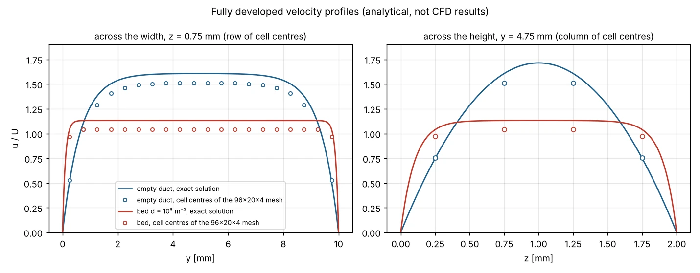
Developed profiles computed with fully_developed.py (lines: exact solution; circles: discrete solution on the 20 × 4 section of the base mesh). In the bed the velocity is almost flat and drops to zero within about 0.1 mm: the first cell, 0.5 mm wide, does not see the layer. Analytical plot, not a CFD result.
Two messages. In the empty duct four cells over the height underestimate the gradient by 12 %: even the d = 0 control case has a large discretisation error. In the bed the error is smaller in percentage because the Darcy term, exact at any resolution, dominates; what is missing is the wall friction of the Brinkman layer, captured only by one third (1.046 against 1.133). A mesh suited to this observable must have wall cells smaller than √K: with 0.1 mm this means grading the mesh towards the walls (section 17 box), not refining it uniformly.
Practical tip · The package run_case.sh script, tested
#!/usr/bin/env bash
# SPDX-License-Identifier: GPL-3.0-or-later
# Execute one fresh case; refuse already-started cases without deleting files.
set -euo pipefail
if [ "$#" -ne 1 ]; then
    printf 'Usage: %s /absolute/path/to/fresh-case\n' "$0" >&2
    exit 2
fi
case_dir="$1"
if [ ! -d "$case_dir" ]; then
    printf 'No such case: %s\n' "$case_dir" >&2
    exit 2
fi
for command_name in blockMesh checkMesh createZones foamRun; do
    command -v "$command_name" >/dev/null 2>&1 || { echo "Missing: $command_name" >&2; exit 2; }
done
if [ -e "$case_dir/log.blockMesh" ] || [ -d "$case_dir/constant/polyMesh" ]; then
    echo "Refusing existing/started case: $case_dir" >&2
    exit 3
fi
cd "$case_dir"
blockMesh > log.blockMesh 2>&1
checkMesh > log.checkMesh 2>&1
createZones > log.createZones 2>&1
# Preserve non-zero exit status and all solver output.
foamRun > log.foamRun 2>&1
printf 'Completed: %s\n' "$case_dir"
Test with the OpenFOAM commands replaced by placeholders (blockMesh, checkMesh, createZones and foamRun that only create the expected files; the postProcessing files are written by extra/make_synthetic_monitors.py and tagged SYNTHETIC: they serve to test the scripts, they are not CFD results). Paths shortened to /home/user.
$ bash run_case.sh "$(pwd)/cases_20_full/U0.0150_D1e08"
Completed: /home/user/OpenFOAM/guide20/exercises/cases_20_full/U0.0150_D1e08
[exit 0]
$ ls cases_20_full/U0.0150_D1e08
0
constant
log.blockMesh
log.checkMesh
log.createZones
log.foamRun
system
[exit 0]
$ bash run_case.sh "$(pwd)/cases_20_full/U0.0150_D1e08"
Refusing existing/started case: /home/user/OpenFOAM/guide20/exercises/cases_20_full/U0.0150_D1e08
[exit 3]- with
set -euo pipefailthe script stops at the first command returning an error code and propagates it: the right behaviour, but it leaves no trace in the case of which step failed (one has to look at the last log written); checkMeshreturns 0 even when it reports failed checks: the mesh quality is read inlog.checkMesh(lineMesh OK.orFailed N mesh checks.);- the command check with
command -vrequires the OpenFOAM environment to be loaded already (source /opt/OpenFOAM-14/etc/bashrc) in the same shell; - a relative path works like an absolute one; the refusal is based on
log.blockMeshorconstant/polyMesh, so a case in whichblockMeshfailed must be copied again from scratch (intended behaviour: no restarts).
Practical tip · run_case_checked.sh: same procedure, with evidence of how it ended
Variant in extra/ with the same arguments and the same refusal of started cases. In addition it writes RUN_STARTED (date, host, OpenFOAM version), records the input hashes with snapshot_inputs.py before the run, checks Mesh OK. and the End line of createZones and foamRun, and closes with RUN_SUCCESS or with RUN_FAILED naming the failed step.
#!/usr/bin/env bash
# SPDX-License-Identifier: GPL-3.0-or-later
# Guide 20: run one fresh reactor case like scripts/run_case.sh (same refusal of
# started cases, same four logs) and leave evidence of how the run ended:
#   RUN_STARTED          date, host, OpenFOAM version, command sequence
#   input_SHA256.txt     hashes of 0/, constant/, system/ before the run
#                        (written by snapshot_inputs.py, if it is found next to this script)
#   RUN_SUCCESS          only if every step returned 0, checkMesh printed
#                        "Mesh OK.", and createZones and foamRun printed "End"
#   RUN_FAILED           the step that failed otherwise
# Usage: bash run_case_checked.sh /absolute/path/to/fresh-case
set -uo pipefail
if [ "$#" -ne 1 ]; then
    printf 'Usage: %s /absolute/path/to/fresh-case\n' "$0" >&2
    exit 2
fi
case_dir="$1"
here="$(cd "$(dirname "$0")" && pwd)"
if [ ! -d "$case_dir/system" ]; then
    printf 'No such case: %s\n' "$case_dir" >&2
    exit 2
fi
for command_name in blockMesh checkMesh createZones foamRun; do
    command -v "$command_name" >/dev/null 2>&1 || { echo "Missing: $command_name (source the OpenFOAM bashrc first)" >&2; exit 2; }
done
for f in log.blockMesh RUN_STARTED RUN_SUCCESS RUN_FAILED constant/polyMesh postProcessing; do
    if [ -e "$case_dir/$f" ]; then
        echo "Refusing existing/started case ($f present): $case_dir" >&2
        exit 3
    fi
done
cd "$case_dir" || exit 2
{
    echo "started  $(date -Iseconds)"
    echo "host     $(hostname)"
    echo "OpenFOAM ${WM_PROJECT_VERSION:-unknown} (${WM_PROJECT_DIR:-?})"
    echo "steps    blockMesh checkMesh createZones foamRun"
} > RUN_STARTED
snap=""
for s in "$here/snapshot_inputs.py" "$here/../exercises/snapshot_inputs.py"; do
    [ -f "$s" ] && snap="$s" && break
done
if [ -n "$snap" ]; then
    python3 "$snap" . --out input_SHA256.txt > /dev/null || { echo "snapshot_inputs" > RUN_FAILED; exit 4; }
fi
fail() { printf '%s\n' "$1" > RUN_FAILED; echo "FAILED at $1: see $case_dir/log.$2" >&2; exit 1; }
blockMesh   > log.blockMesh   2>&1 || fail blockMesh blockMesh
checkMesh   > log.checkMesh   2>&1 || fail checkMesh checkMesh
grep -q '^Mesh OK\.' log.checkMesh || fail 'checkMesh (no "Mesh OK.")' checkMesh
createZones > log.createZones 2>&1 || fail createZones createZones
grep -q '^End' log.createZones || fail 'createZones (no End line)' createZones
foamRun     > log.foamRun     2>&1 || fail foamRun foamRun
grep -q '^End' log.foamRun || fail 'foamRun (no End line)' foamRun
date -Iseconds > RUN_SUCCESS
printf 'Completed: %s\n' "$case_dir"
Test with the OpenFOAM commands replaced by placeholders (blockMesh, checkMesh, createZones and foamRun that only create the expected files; the postProcessing files are written by extra/make_synthetic_monitors.py and tagged SYNTHETIC: they serve to test the scripts, they are not CFD results). Paths shortened to /home/user.
$ for c in run01/U*; do bash extra/run_case_checked.sh "$(pwd)/$c" || break; done
Completed: /home/user/OpenFOAM/guide20/run01/U0.0075_D0e00
Completed: /home/user/OpenFOAM/guide20/run01/U0.0075_D1e08
Completed: /home/user/OpenFOAM/guide20/run01/U0.0075_D2e08
Completed: /home/user/OpenFOAM/guide20/run01/U0.0075_D5e07
Completed: /home/user/OpenFOAM/guide20/run01/U0.0150_D0e00
Completed: /home/user/OpenFOAM/guide20/run01/U0.0150_D1e08
Completed: /home/user/OpenFOAM/guide20/run01/U0.0150_D2e08
Completed: /home/user/OpenFOAM/guide20/run01/U0.0150_D5e07
Completed: /home/user/OpenFOAM/guide20/run01/U0.0300_D0e00
Completed: /home/user/OpenFOAM/guide20/run01/U0.0300_D1e08
Completed: /home/user/OpenFOAM/guide20/run01/U0.0300_D2e08
Completed: /home/user/OpenFOAM/guide20/run01/U0.0300_D5e07
[exit 0]
$ bash extra/run_case_checked.sh "$(pwd)/run01/U0.0150_D1e08"
Refusing existing/started case (log.blockMesh present): /home/user/OpenFOAM/guide20/run01/U0.0150_D1e08
[exit 3]
$ ls run01/U0.0150_D1e08 run01/U0.0150_D1e08/postProcessing
run01/U0.0150_D1e08:
0
RUN_STARTED
RUN_SUCCESS
constant
input_SHA256.txt
log.blockMesh
log.checkMesh
log.createZones
log.foamRun
postProcessing
system

run01/U0.0150_D1e08/postProcessing:
centreline
inletFlowRate
inletPressure
outletFlowRate
pDown
pUp
qBed
qDown
qUp
[exit 0]
$ cat run01/U0.0150_D1e08/RUN_STARTED run01/U0.0150_D1e08/RUN_SUCCESS
started  2026-11-01T07:38:20+01:00
host     vm
OpenFOAM 14 (/opt/OpenFOAM-14)
steps    blockMesh checkMesh createZones foamRun
2026-11-01T07:38:20+01:00
[exit 0]
To see how many cells createZones selected without opening ParaView, OpenFOAM 14 provides the print generator: appended to system/createZonesDict (in a new copy of the case) it prints in the log the number of cells, volume, centroid and bounding box of the zone. Expect 2560 cells and 8·10⁻⁷ m³ with the base mesh.
printBed
{
    type        print;
    zone        reactorBed;
}
9. Running an isolated parameter campaign
prepare_campaign.py creates 12 independent cases: three inlet velocities for four Darcy coefficients, including an unobstructed reference with d = 0. Existing destinations are never overwritten. --quick builds only the three cases having d = 10⁸ m⁻² for an initial smoke test.
# This Python command also runs locally on Windows (inside exercises/).
python prepare_campaign.py --out cases_trial --quick
# Transfer exercises/ to Linux via FileZilla, then:
source /opt/OpenFOAM-14/etc/bashrc
python3 prepare_campaign.py --out cases_20_full
bash run_case.sh "$(pwd)/cases_20_full/U0.0150_D1e08"run_case.sh deliberately refuses a case containing an existing mesh or an earlier meshing log. It is not a restart tool. To repeat the experiment, prepare a newly named case and retain the previous version for traceability.
Practical tip · The prepare_campaign.py script, tested
#!/usr/bin/env python3
# SPDX-License-Identifier: GPL-3.0-or-later
"""Create independent reactor cases without changing the template or older runs."""
import argparse
import csv
from pathlib import Path
import re
import shutil

ROOT = Path(__file__).resolve().parent
TEMPLATE = ROOT / "template"
VELOCITIES = (0.0075, 0.015, 0.03)
RESISTANCES = (0.0, 5e7, 1e8, 2e8)


def replace_one(path: Path, pattern: str, replacement: str) -> None:
    text = path.read_text(encoding="utf-8")
    result, count = re.subn(pattern, replacement, text, flags=re.MULTILINE)
    if count != 1:
        raise ValueError(f"Expected exactly one match in {path}: got {count}")
    path.write_text(result, encoding="utf-8", newline="\n")


def main() -> None:
    parser = argparse.ArgumentParser(description=__doc__)
    parser.add_argument("--out", type=Path, required=True, help="New destination directory; must not exist")
    parser.add_argument("--quick", action="store_true", help="Only 3 baseline velocity cases")
    args = parser.parse_args()
    dest = args.out.resolve()
    if dest.exists():
        parser.error(f"Destination already exists (will not overwrite): {dest}")
    if not TEMPLATE.is_dir():
        parser.error(f"Missing template: {TEMPLATE}")
    if not args.quick and len(VELOCITIES) * len(RESISTANCES) != 12:
        raise AssertionError("Unexpected campaign dimensions")
    rows = []
    values = (1e8,) if args.quick else RESISTANCES
    try:
        dest.mkdir(parents=True)
        for vel in VELOCITIES:
            for d in values:
                case_id = f"U{vel:.4f}_D{d:.0e}".replace("+", "")
                target = dest / case_id
                shutil.copytree(TEMPLATE, target)
                replace_one(target / "0" / "U", r"(?m)^internalField uniform \([^\n]+\);$", f"internalField uniform ({vel:.5f} 0 0);")
                replace_one(target / "0" / "U", r"(?m)^\s*value uniform \(0\.015 0 0\);$", f"        value uniform ({vel:.5f} 0 0);")
                replace_one(target / "constant" / "fvModels", r"(?m)^\s*D 1e8;$", f"        D {d:.8g};")
                rows.append({"case_id": case_id, "velocity_in_m_s": f"{vel:.5f}", "d_m_inv2": f"{d:.8g}", "source": "guide20"})
        with (dest / "manifest.csv").open("w", newline="", encoding="utf-8") as f:
            w = csv.DictWriter(f, fieldnames=list(rows[0])); w.writeheader(); w.writerows(rows)
    except Exception:
        # Leave the incomplete destination intact for inspection; never delete work.
        raise
    print(f"Created {len(rows)} independent cases at {dest}")


if __name__ == "__main__":
    main()
Test on the package copied to the server (no OpenFOAM command involved):
$ python3 prepare_campaign.py --out cases_trial --quick
Created 3 independent cases at /home/user/OpenFOAM/guide20/exercises/cases_trial
[exit 0]
$ cat cases_trial/manifest.csv
case_id,velocity_in_m_s,d_m_inv2,source
U0.0075_D1e08,0.00750,1e+08,guide20
U0.0150_D1e08,0.01500,1e+08,guide20
U0.0300_D1e08,0.03000,1e+08,guide20
[exit 0]
$ python3 prepare_campaign.py --out cases_20_full
Created 12 independent cases at /home/user/OpenFOAM/guide20/exercises/cases_20_full
[exit 0]
$ ls cases_20_full
U0.0075_D0e00
U0.0075_D1e08
U0.0075_D2e08
U0.0075_D5e07
U0.0150_D0e00
U0.0150_D1e08
U0.0150_D2e08
U0.0150_D5e07
U0.0300_D0e00
U0.0300_D1e08
U0.0300_D2e08
U0.0300_D5e07
manifest.csv
[exit 0]
$ diff template/0/U cases_20_full/U0.0300_D2e08/0/U
10c10
< internalField uniform (0.015 0 0);
---
> internalField uniform (0.03000 0 0);
16c16
<         value uniform (0.015 0 0);
---
>         value uniform (0.03000 0 0);
[exit 1]
$ diff template/constant/fvModels cases_20_full/U0.0075_D0e00/constant/fvModels
17,18c17
<
<         D 1e8;
---
>         D 0;
[exit 1]
$ python3 prepare_campaign.py --out cases_20_full
usage: prepare_campaign.py [-h] --out OUT [--quick]
prepare_campaign.py: error: Destination already exists (will not overwrite): /home/user/OpenFOAM/guide20/exercises/cases_20_full
[exit 2]- names follow
f"U{vel:.4f}_D{d:.0e}"without the + sign:D0e00,D5e07,D1e08,D2e08; inmanifest.csvd is written as1e+08; - the replacement of
D 1e8;uses^\s*D 1e8;$in multiline mode:\s*also swallows the preceding blank line, which disappears (visible in thediff). It is only cosmetic; the same pattern requiresD 1e8;to appear exactly once, so a hand-modifiedfvModelsis refused with a clear error; - velocities are written with five decimals (
0.03000): enough for the guide values, but velocities smaller than 10⁻⁵ m/s would be rounded; - in case of an error halfway the destination folder stays incomplete and is not deleted: inspect it, rename it, then run again with a new name.
Deep dive · The expected values of the campaign before computing it
With the campaign prepared, case_estimates.py on all the cases gives the table of predictions: Darcy-only ΔP (guide formula), exact developed ΔP between the planes, time steps, analytical τ and X. Save it in the report before the runs: it is the yardstick to recognise a wrong case (missing zone, d not replaced, wrong flow rate).
$ python3 extra/case_estimates.py run01/U*
case                          cells   U m/s   d 1/m2     Re  Darcy Pa dP35-85 Pa  steps  tau s    X %
U0.0075_D0e00                  7680  0.0075        0   25.0     0.000      1.287   1600  3.733  17.03
U0.0075_D1e08                  7680  0.0075    1e+08   25.0    30.000     34.250   1600  3.733  17.03
U0.0075_D2e08                  7680  0.0075    2e+08   25.0    60.000     65.730   1600  3.733  17.03
U0.0075_D5e07                  7680  0.0075    5e+07   25.0    15.000     18.213   1600  3.733  17.03
U0.0150_D0e00                  7680  0.0150        0   50.0     0.000      2.575   1600  1.867   8.91
U0.0150_D1e08                  7680  0.0150    1e+08   50.0    60.000     68.500   1600  1.867   8.91
U0.0150_D2e08                  7680  0.0150    2e+08   50.0   120.000    131.459   1600  1.867   8.91
U0.0150_D5e07                  7680  0.0150    5e+07   50.0    30.000     36.426   1600  1.867   8.91
U0.0300_D0e00                  7680  0.0300        0  100.0     0.000      5.149   1600  0.933   4.56
U0.0300_D1e08                  7680  0.0300    1e+08  100.0   120.000    137.000   1600  0.933   4.56
U0.0300_D2e08                  7680  0.0300    2e+08  100.0   240.000    262.918   1600  0.933   4.56
U0.0300_D5e07                  7680  0.0300    5e+07  100.0    60.000     72.853   1600  0.933   4.56
[exit 0]
Reading: at fixed velocity ΔP is linear in d plus a constant (the duct); at fixed d it is proportional to U. The ratio between the exact and the Darcy column decreases with d (1.21 for 5·10⁷, 1.10 for 2·10⁸ including the 10 mm of duct) because the Brinkman layer gets thinner. The 3 × 4 factorial table allows the two effects to be separated with the regressions of Exercise B; the d = 0 case at every velocity is the control that makes the insert contribution measurable.
10. Physical time, stability and convergence
The provided model is transient (Euler, PIMPLE, adjustTimeStep yes, maxCo 0.5). It begins from a uniform state, so a real transient must pass before reporting a quasi-steady outcome. endTime = 16 s is a starting demonstration parameter, not proof that a stationary state has been reached.
Specify a final measurement window and check for drifts in pressure loss, flow rates and selected velocity probes. Inspect Courant numbers, solver residuals, continuity errors and elapsed wall-clock time. If the run does not reach a usable quasi-steady state, continue in a documented new experiment or version rather than silently using the last saved field.
Deep dive · How much simulated time is really needed: viscous, Darcy and flow-through scales
The case starts with uniform U everywhere. For an incompressible fluid the pressure adapts instantaneously, and the velocity field settles with three scales:
- viscous diffusion in the section: τν = 1/(νπ²(1/W² + 1/H²)) = 0.39 s, the decay time of the slowest mode; after 5τν ≈ 2 s the disturbance is below 1 %;
- Darcy relaxation in the bed: 1/(νd) = 0.005–0.02 s, practically instantaneous;
- convection of the development zone: Le/U ≈ 0.7 s for all three velocities.
For ΔP and Q, therefore, 16 s are 8 to 40 times what is needed: the final window (for example 12–16 s) must show a drift comparable with the solver tolerance. A transported scalar is different (the reaction of section 20): the front crosses the domain in L/U = 16, 8 and 4 s, and the steady state takes several flow-through times; add_reaction_tracer.py therefore raises endTime to 4 L/U.
The step is always 0.01 s (maxDeltaT): the maximum Courant number, computed with the duct centre velocity (1.715 U), is 0.10, 0.21 and 0.41. On the fine mesh of Exercise C (Δx = 0.625 mm) the Courant number at 0.01 s is 0.41 for U = 0.015 and the step does not change; for U = 0.03 the limit becomes maxCo (Δt ≈ 0.006 s, about 2600 steps). Since only the steady state matters, time accuracy is irrelevant; a steady formulation (SIMPLE with steadyState) would reach the same result with fewer iterations, but would change the controls and convergence criteria of the guide: if used, it must be documented as a variant.
Practical tip · How to demonstrate that the steady state is reached
- define the window before looking at the data (for example the last 4 s) and compute the relative drift between its two halves:
extract_measurements.pyreports it for ΔP and for the inlet Q (columnsdrift_dPanddrift_q_in); - a drift below 10⁻⁴ is consistent with
tolerance 1e-06on pressure; values of order 10⁻² indicate a non-steady or oscillating computation; - in the log,
time step continuity errorsmust stay at 10⁻⁹ or below (sum local);Courant Number mean/maxconfirms the step; - the initial residuals of p and U (
postProcessing/residuals) fall and level off: in a transient run that has reached the steady state the initial residual of every step stays small and constant; - if the run is extended, do it in a copy or with a documented
startTime, as the guide requires:extract_measurements.pyjoinspostProcessingfolders with different start times, giving precedence to the most recent one on overlapping times.
11. Quantitative measurements in Windows ParaView
Connect the Windows ParaView client to Linux pvserver as explained in Guide 3. Measure cross-sections at x = 35 mm and 85 mm; these are outside the bed and therefore include both bed resistance and the ordinary fluid losses between the stations. Obtain area-averaged kinematic pressure on both cross-sections and surface-integrated volumetric flux at inlet and outlet.
Keep outward surface normals and signed volumetric fluxes straight: a boundary inlet generally has negative signed outward flow, and an outlet has positive. The supplied CSV template requests positive magnitudes q_in_abs_m3_s and q_out_abs_m3_s.
Only enter actual measured values into measurements_template.csv. Blank values are intentional, preventing invented data from being mistaken for a successful CFD calculation. The analysis program refuses a file with no observations.
Deep dive · Measurements written by the solver: add_monitors.py and the planes generated in OpenFOAM 14
The quantities the guide extracts by hand in ParaView can be written at every step by function objects, on the same sections. Two details of the source determine the configuration. First, surfaceFieldValue reads a volume field only on boundary faces: on internal faces it stops with an error (surfaceFieldValueTemplates.C):
template<class Type>
Foam::tmp<Foam::Field<Type>>
Foam::functionObjects::fieldValues::surfaceFieldValue::filterField
(
    const VolField<Type>& field
) const
{
    tmp<Field<Type>> tvalues(new Field<Type>(faceId_.size()));
    Field<Type>& values = tvalues.ref();

    forAll(values, i)
    {
        const label facei = faceId_[i];
        const label patchi = facePatchId_[i];

        if (patchi >= 0)
        {
            values[i] = field.boundaryField()[patchi][facei];
        }
        else
        {
            FatalErrorInFunction
                << type() << " " << name() << ": "
                << selectionTypeNames[selectionType_]
                << "(" << selectionName_.c_str() << "):"
                << nl
                << "    Unable to process internal faces for volume field "
                << field.name() << nl << abort(FatalError);
        }
    }

    return tvalues;
}
this is why p is first interpolated to the faces by the surfaceInterpolate function object (field pf), while for the flow rate the flux phi is used directly. Second, in OpenFOAM 14 the faceZone selection accepts a generation dictionary (generatedFaceZone.H): the plane type picks the faces between cell centres on opposite sides of the plane and provides the orientation, so orientedSum(phi) is positive along the normal. There is no need to touch createZonesDict. With the base mesh the planes at 35, 60 and 85 mm lie exactly on faces (Δx = 1.25 mm) and contain 80 faces for 2.0·10⁻⁵ m²: writeArea and writeNumberOfFaces make this checkable.
The script:
#!/usr/bin/env python3
# SPDX-License-Identifier: GPL-3.0-or-later
"""Install the Guide 20 measurement monitors in NEW, never-run reactor cases.

The template has no system/functions: this script writes one (with the FoamFile
header OpenFOAM 14 requires), so that the quantities of sections 11-12 are
recorded by the solver at every time step instead of being picked by hand in
ParaView at the end:

  inletFlowRate, outletFlowRate   sum(phi) on the patches [m3/s]
                                  (inlet negative, outlet positive)
  inletPressure                   areaAverage(p) on the inlet [m2/s2]
  pFace                           surface interpolate of p (pf), needed because
                                  surfaceFieldValue cannot read a volume field
                                  on internal faces
  pUp, pDown                      areaAverage(pf) on the planes x = 35 and 85 mm
  qUp, qBed, qDown                orientedSum(phi) on the planes x = 35, 60 and
                                  85 mm, positive along +x
  centreline                      p and U along y = 5 mm, z = 1 mm (241 points)
  profileDuct, profileBed         U across the width at x = 20 and 60 mm
  residuals                       initial residuals of p and U

The planes are generated by the function objects themselves (OpenFOAM 14
faceZone dictionary, type plane): createZonesDict and the physics of the case
are not changed. Cases with logs, a mesh, postProcessing or an existing
system/functions are refused and nothing is written.

Usage: python3 add_monitors.py CASE [CASE ...]      (or CAMPAIGN_DIR/U*)
       python3 add_monitors.py --print              (show the file)
       options: --x-up 0.035 --x-down 0.085 --x-bed 0.06
"""
import argparse, glob, os, sys

MARK = '// Guide 20 monitors (written by add_monitors.py)'
HEADER = r'''/*--------------------------------*- C++ -*----------------------------------*\
  =========                 |
  \\      /  F ield         | OpenFOAM: The Open Source CFD Toolbox
   \\    /   O peration     | Website:  https://openfoam.org
    \\  /    A nd           | Version:  14
     \\/     M anipulation  |
\*---------------------------------------------------------------------------*/
FoamFile
{
    format      ascii;
    class       dictionary;
    location    "system";
    object      functions;
}
// * * * * * * * * * * * * * * * * * * * * * * * * * * * * * * * * * * * * * //
'''


def plane(name, x, op, field):
    return f'''{name}
{{
    type            surfaceFieldValue;
    libs            ("libfieldFunctionObjects.so");
    writeControl    timeStep;
    writeInterval   1;
    writeFields     false;
    writeArea       yes;
    writeNumberOfFaces yes;
    faceZone
    {{
        type        plane;
        point       ({x:g} 0.005 0.001);
        normal      (1 0 0);
    }}
    operation       {op};
    fields          ({field});
}}
'''


def body(xu, xd, xb):
    return (MARK + f'''
// Planes x = {xu*1e3:g} mm (upstream), {xb*1e3:g} mm (inside the bed), {xd*1e3:g} mm (downstream).

// Volumetric flow rates on the patches [m3/s]: inlet negative, outlet positive.
#includeFunc patchFlowRate(name=inletFlowRate, patch=inlet)
#includeFunc patchFlowRate(name=outletFlowRate, patch=outlet)

// Area-averaged kinematic pressure on the inlet [m2/s2] (outlet is fixed at 0).
#includeFunc patchAverage(name=inletPressure, patch=inlet, p)

// Face values of p: surfaceFieldValue reads volume fields only on boundary faces.
pFace
{{
    type            surfaceInterpolate;
    libs            ("libfieldFunctionObjects.so");
    field           p;
    result          pf;
    executeControl  timeStep;
    writeControl    writeTime;
}}

''' + plane('pUp', xu, 'areaAverage', 'pf') + '\n' + plane('pDown', xd, 'areaAverage', 'pf') + '\n'
            + plane('qUp', xu, 'orientedSum', 'phi') + '\n' + plane('qBed', xb, 'orientedSum', 'phi') + '\n'
            + plane('qDown', xd, 'orientedSum', 'phi') + f'''
// Axial profile of p and U on the channel axis and two transverse velocity profiles.
#includeFunc graphUniform(name=centreline, start=(0 0.005 0.001), end=(0.12 0.005 0.001), nPoints=241, axis=x, p, U)
#includeFunc graphUniform(name=profileDuct, start=(0.02 0 0.001), end=(0.02 0.01 0.001), nPoints=101, axis=y, U)
#includeFunc graphUniform(name=profileBed, start=({xb:g} 0 0.001), end=({xb:g} 0.01 0.001), nPoints=101, axis=y, U)

// Initial residuals at every time step.
#includeFunc residuals(p, U)
''')


def check(case):
    if not all(os.path.isdir(os.path.join(case, d)) for d in ('0', 'constant', 'system')):
        return 'not an OpenFOAM case'
    bad = [os.path.basename(p) for p in glob.glob(os.path.join(case, 'log.*'))]
    bad += [f for f in ('postProcessing', 'constant/polyMesh', 'system/functions', 'RUN_STARTED') if os.path.exists(os.path.join(case, f))]
    if bad:
        return 'already started, meshed or with functions (' + ', '.join(bad) + ')'
    if not os.path.isfile(os.path.join(case, 'constant', 'fvModels')):
        return 'constant/fvModels missing: not a Guide 20 case'
    return None


def main():
    ap = argparse.ArgumentParser(description=__doc__.split('\n')[0])
    ap.add_argument('cases', nargs='*')
    ap.add_argument('--print', action='store_true')
    ap.add_argument('--x-up', type=float, default=0.035)
    ap.add_argument('--x-down', type=float, default=0.085)
    ap.add_argument('--x-bed', type=float, default=0.06)
    a = ap.parse_args()
    text = HEADER + '\n' + body(a.x_up, a.x_down, a.x_bed) + '\n// ************************************************************************* //\n'
    if a.print:
        sys.stdout.write(text)
        return
    if not a.cases:
        sys.exit(__doc__)
    cases = [c for c in a.cases if os.path.isdir(c)]
    errors = {c: check(c) for c in cases}
    errors.update({c: 'not a directory' for c in a.cases if c not in cases})
    for c, e in errors.items():
        if e:
            print(f'{c}: {e}')
    if any(errors.values()):
        sys.exit('nothing changed')
    for c in cases:
        with open(os.path.join(c, 'system', 'functions'), 'x', encoding='utf-8', newline='\n') as f:
            f.write(text)
        print(f'{c}: system/functions written (monitors at x = {a.x_up:g}, {a.x_bed:g}, {a.x_down:g} m)')


if __name__ == '__main__':
    main()
The system/functions file it writes (included in the archive as extra/functions_guide20):
/*--------------------------------*- C++ -*----------------------------------*\
  =========                 |
  \\      /  F ield         | OpenFOAM: The Open Source CFD Toolbox
   \\    /   O peration     | Website:  https://openfoam.org
    \\  /    A nd           | Version:  14
     \\/     M anipulation  |
\*---------------------------------------------------------------------------*/
FoamFile
{
    format      ascii;
    class       dictionary;
    location    "system";
    object      functions;
}
// * * * * * * * * * * * * * * * * * * * * * * * * * * * * * * * * * * * * * //

// Guide 20 monitors (written by add_monitors.py)
// Planes x = 35 mm (upstream), 60 mm (inside the bed), 85 mm (downstream).

// Volumetric flow rates on the patches [m3/s]: inlet negative, outlet positive.
#includeFunc patchFlowRate(name=inletFlowRate, patch=inlet)
#includeFunc patchFlowRate(name=outletFlowRate, patch=outlet)

// Area-averaged kinematic pressure on the inlet [m2/s2] (outlet is fixed at 0).
#includeFunc patchAverage(name=inletPressure, patch=inlet, p)

// Face values of p: surfaceFieldValue reads volume fields only on boundary faces.
pFace
{
    type            surfaceInterpolate;
    libs            ("libfieldFunctionObjects.so");
    field           p;
    result          pf;
    executeControl  timeStep;
    writeControl    writeTime;
}

pUp
{
    type            surfaceFieldValue;
    libs            ("libfieldFunctionObjects.so");
    writeControl    timeStep;
    writeInterval   1;
    writeFields     false;
    writeArea       yes;
    writeNumberOfFaces yes;
    faceZone
    {
        type        plane;
        point       (0.035 0.005 0.001);
        normal      (1 0 0);
    }
    operation       areaAverage;
    fields          (pf);
}

pDown
{
    type            surfaceFieldValue;
    libs            ("libfieldFunctionObjects.so");
    writeControl    timeStep;
    writeInterval   1;
    writeFields     false;
    writeArea       yes;
    writeNumberOfFaces yes;
    faceZone
    {
        type        plane;
        point       (0.085 0.005 0.001);
        normal      (1 0 0);
    }
    operation       areaAverage;
    fields          (pf);
}

qUp
{
    type            surfaceFieldValue;
    libs            ("libfieldFunctionObjects.so");
    writeControl    timeStep;
    writeInterval   1;
    writeFields     false;
    writeArea       yes;
    writeNumberOfFaces yes;
    faceZone
    {
        type        plane;
        point       (0.035 0.005 0.001);
        normal      (1 0 0);
    }
    operation       orientedSum;
    fields          (phi);
}

qBed
{
    type            surfaceFieldValue;
    libs            ("libfieldFunctionObjects.so");
    writeControl    timeStep;
    writeInterval   1;
    writeFields     false;
    writeArea       yes;
    writeNumberOfFaces yes;
    faceZone
    {
        type        plane;
        point       (0.06 0.005 0.001);
        normal      (1 0 0);
    }
    operation       orientedSum;
    fields          (phi);
}

qDown
{
    type            surfaceFieldValue;
    libs            ("libfieldFunctionObjects.so");
    writeControl    timeStep;
    writeInterval   1;
    writeFields     false;
    writeArea       yes;
    writeNumberOfFaces yes;
    faceZone
    {
        type        plane;
        point       (0.085 0.005 0.001);
        normal      (1 0 0);
    }
    operation       orientedSum;
    fields          (phi);
}

// Axial profile of p and U on the channel axis and two transverse velocity profiles.
#includeFunc graphUniform(name=centreline, start=(0 0.005 0.001), end=(0.12 0.005 0.001), nPoints=241, axis=x, p, U)
#includeFunc graphUniform(name=profileDuct, start=(0.02 0 0.001), end=(0.02 0.01 0.001), nPoints=101, axis=y, U)
#includeFunc graphUniform(name=profileBed, start=(0.06 0 0.001), end=(0.06 0.01 0.001), nPoints=101, axis=y, U)

// Initial residuals at every time step.
#includeFunc residuals(p, U)

// ************************************************************************* //
Test with the OpenFOAM commands replaced by placeholders (blockMesh, checkMesh, createZones and foamRun that only create the expected files; the postProcessing files are written by extra/make_synthetic_monitors.py and tagged SYNTHETIC: they serve to test the scripts, they are not CFD results). Paths shortened to /home/user.
$ python3 extra/add_monitors.py run01/U*
run01/U0.0075_D0e00: system/functions written (monitors at x = 0.035, 0.06, 0.085 m)
run01/U0.0075_D1e08: system/functions written (monitors at x = 0.035, 0.06, 0.085 m)
run01/U0.0075_D2e08: system/functions written (monitors at x = 0.035, 0.06, 0.085 m)
run01/U0.0075_D5e07: system/functions written (monitors at x = 0.035, 0.06, 0.085 m)
run01/U0.0150_D0e00: system/functions written (monitors at x = 0.035, 0.06, 0.085 m)
run01/U0.0150_D1e08: system/functions written (monitors at x = 0.035, 0.06, 0.085 m)
run01/U0.0150_D2e08: system/functions written (monitors at x = 0.035, 0.06, 0.085 m)
run01/U0.0150_D5e07: system/functions written (monitors at x = 0.035, 0.06, 0.085 m)
run01/U0.0300_D0e00: system/functions written (monitors at x = 0.035, 0.06, 0.085 m)
run01/U0.0300_D1e08: system/functions written (monitors at x = 0.035, 0.06, 0.085 m)
run01/U0.0300_D2e08: system/functions written (monitors at x = 0.035, 0.06, 0.085 m)
run01/U0.0300_D5e07: system/functions written (monitors at x = 0.035, 0.06, 0.085 m)
[exit 0]
$ python3 extra/add_monitors.py run01/U0.0150_D1e08
run01/U0.0150_D1e08: already started, meshed or with functions (system/functions)
nothing changed
[exit 1]
$ ls run01/U0.0150_D1e08 run01/U0.0150_D1e08/postProcessing
run01/U0.0150_D1e08:
0
RUN_STARTED
RUN_SUCCESS
constant
input_SHA256.txt
log.blockMesh
log.checkMesh
log.createZones
log.foamRun
postProcessing
system
run01/U0.0150_D1e08/postProcessing:
centreline
inletFlowRate
inletPressure
outletFlowRate
pDown
pUp
qBed
qDown
qUp
[exit 0]
$ head -4 run01/U0.0150_D1e08/postProcessing/pUp/0/surfaceFieldValue.dat
# SYNTHETIC data written by make_synthetic_monitors.py - NOT OpenFOAM output
# Time faces area areaAverage(pf)
0.01 8.00000000e+01 2.00000000e-05 1.71972850e-03
0.02 8.00000000e+01 2.00000000e-05 3.54788922e-03
[exit 0]The files go to postProcessing/<name>/0/surfaceFieldValue.dat (columns: time, faces, area, value) and, for the graphs, to postProcessing/centreline/<time>/line.xy. The script refuses cases already started or with an existing system/functions; run it after prepare_campaign.py and before run_case.sh.
Practical tip · When measuring in ParaView: procedure and pitfalls
- Slice with normal (1, 0, 0) and origin (0.035, 0.005, 0.001), then Integrate Variables: the result contains the area and the integrals of the fields; with Divide Cell Data By Volume the cell data become area averages. Repeat at 0.085 m;
- always check the returned area: it must be 2.0·10⁻⁵ m². The 35 and 85 mm planes coincide with cell faces; if the cut produces duplicate or missing polygons the area is wrong, and it is better to shift the plane by a small fraction of a cell (for example 35.1 mm), noting it;
- for the flow rate integrate Ux over the slice (with a Calculator if the normal is not an axis); with data interpolated to points the velocity near the walls is averaged with the zero wall value and the flow rate can come out a few percent low on a mesh with four cells in height: for the balance use the boundary fluxes (
phi), not the slices; - the pressure in the files is kinematic: note the time step used and save the
.pvsmstate together with the screenshots with axes and scale; - Plot Over Line from (0, 0.005, 0.001) to (0.12, 0.005, 0.001) shows the pressure along the axis: three straight stretches with different slopes (duct, bed, duct) separate the contributions at a glance.
12. Pressure conversion and continuity error
Turn the kinematic pressure difference into pascals and compute a simple flow-balance error:
A 1% flow-balance flag is provided as a teaching default, not a universal acceptance criterion. The acceptable tolerance must reflect the scientific purpose and achieved convergence. Distinguish the measured station-to-station pressure difference from a Darcy-only estimate of the additional porous loss.
Deep dive · Mass balance with finite volumes: why 1 % is a loose threshold
In an incompressible finite-volume solver continuity is imposed cell by cell by the pressure equation: the sum of the fluxes phi over each cell is zero up to the solver tolerance (here 10⁻⁶ on the normalised residual, relTol 0 at the last corrector). Summing over the cells, the difference between inlet and outlet flow rate computed from phi is of order 10⁻⁶ relative or less; the log reports it as time step continuity errors.
Three practical rules follow: with the boundary flow rates of add_monitors.py a balance worse than 10⁻⁴ flags a problem (non-converged run, wrong patch); with ParaView measurements on interpolated slices the guide’s 1 % is reasonable, because the error belongs to interpolation, not to the solver; in any case also compare Qin with A·Uin: the q_in_vs_AU column of extract_measurements.py must be zero up to rounding, and immediately reveals a case with a wrong velocity.
The flow rates on the internal planes (qUp, qBed, qDown) must coincide with the boundary ones: they are an independent check of the zone and of the plane orientation.
Practical tip · extract_measurements.py: from postProcessing to the measurements CSV, with the evidence
The script fills the file in the format of measurements_template.csv (ready for analyze_measurements.py) with the averages over the final window and writes an evidence file next to it: samples, drift, faces and area of the plane, internal flow rates, Qin/(A·U) − 1, balance, axial gradients estimated on the axis profile (duct 15–30 mm, bed 50–70 mm) and, if the tracer of section 20 is present, XCFD.
#!/usr/bin/env python3
# SPDX-License-Identifier: GPL-3.0-or-later
"""Fill the Guide 20 measurements CSV from the monitors written by add_monitors.py.

For every case of a campaign (manifest.csv of prepare_campaign.py, or --cases)
it reads postProcessing/ and averages, over the final window of simulated time
(--window seconds, default 4: t = 12-16 s with the template), the kinematic
pressures on the 35 and 85 mm planes and the absolute inlet and outlet flow
rates. It writes:

  --out       the measurements file in the format of measurements_template.csv,
              ready for analyze_measurements.py (rho from --rho, nu from the case)
  --evidence  the checks that justify each number: samples in the window,
              relative drift between the two halves of the window, number of
              faces and area of each plane, flow rates on the internal planes,
              Q_in against A*U_in, axial pressure gradients fitted on the
              centreline graph (duct 15-30 mm, bed 50-70 mm) and, if the case
              has the reacting tracer, X_CFD = 1 - outletC/inletC

Cases without monitors are listed and skipped. Existing outputs are never
overwritten.

Usage: python3 extract_measurements.py CAMPAIGN_DIR --out measurements_cfd.csv
           --evidence evidence.csv [--cases U0.0150_D1e08 ...] [--rho 1000] [--window 4]
"""
import argparse, csv, glob, math, os, re, sys

AREA = 0.01 * 0.002


def series(case, name):
    """(time, columns...) rows of postProcessing/name/*/*.dat; later start times win on overlaps."""
    dirs = sorted(glob.glob(os.path.join(case, 'postProcessing', name, '*')), key=lambda p: float(os.path.basename(p)))
    rows = []
    for d in dirs:
        part = []
        for f in sorted(glob.glob(os.path.join(d, '*.dat'))):
            for line in open(f, encoding='utf-8'):
                if line.startswith('#') or not line.strip():
                    continue
                v = line.replace('(', ' ').replace(')', ' ').split()
                part.append([float(x) for x in v])
        if part:
            t0 = part[0][0]
            rows = [r for r in rows if r[0] < t0] + part
    return rows


def window(rows, width, col=-1):
    if not rows:
        return None
    tend = rows[-1][0]
    w = [r for r in rows if r[0] >= tend - width - 1e-12]
    vals = [r[col] for r in w]
    half = len(vals) // 2
    mean = sum(vals) / len(vals)
    drift = (sum(vals[half:]) / max(len(vals) - half, 1) - sum(vals[:half]) / max(half, 1)) / abs(mean) if half and mean else float('nan')
    return dict(mean=mean, drift=drift, n=len(vals), t0=w[0][0], t1=tend, row=w[-1])


def last_graph(case, name):
    dirs = sorted(glob.glob(os.path.join(case, 'postProcessing', name, '*')), key=lambda p: float(os.path.basename(p)))
    for d in reversed(dirs):
        for f in glob.glob(os.path.join(d, '*.xy')):
            head, data = None, []
            for line in open(f, encoding='utf-8'):
                if line.startswith('#'):
                    head = line[1:].split()
                elif line.strip():
                    data.append([float(v) for v in line.split()])
            return head, data, float(os.path.basename(d))
    return None, [], None


def slope(pts):
    n = len(pts)
    if n < 3:
        return float('nan')
    mx = sum(x for x, _ in pts) / n
    my = sum(y for _, y in pts) / n
    sxx = sum((x - mx) ** 2 for x, _ in pts)
    return sum((x - mx) * (y - my) for x, y in pts) / sxx


def case_values(case):
    u = open(os.path.join(case, '0', 'U'), encoding='utf-8').read()
    U = float(re.search(r'inlet\s*\{[^}]*value\s+uniform\s*\(\s*([-+0-9.eE]+)', u, re.S).group(1))
    fv = re.sub(r'//.*', '', open(os.path.join(case, 'constant', 'fvModels.noReaction') if os.path.exists(os.path.join(case, 'constant', 'fvModels.noReaction'))
                else os.path.join(case, 'constant', 'fvModels'), encoding='utf-8').read())
    d = float(re.search(r'(?m)^\s*D\s+([-+0-9.eE]+)\s*;', fv).group(1))
    nu = float(re.search(r'(?m)^\s*nu\s+([-+0-9.eE]+)\s*;', open(os.path.join(case, 'constant', 'physicalProperties'), encoding='utf-8').read()).group(1))
    return U, d, nu


def main():
    ap = argparse.ArgumentParser(description=__doc__.split('\n')[0])
    ap.add_argument('campaign')
    ap.add_argument('--cases', nargs='+')
    ap.add_argument('--out', required=True)
    ap.add_argument('--evidence', required=True)
    ap.add_argument('--rho', type=float, default=1000.0)
    ap.add_argument('--window', type=float, default=4.0)
    a = ap.parse_args()
    for p in (a.out, a.evidence):
        if os.path.exists(p):
            sys.exit(f'{p} exists: refusing to overwrite')
    if a.cases:
        ids = a.cases
    else:
        man = os.path.join(a.campaign, 'manifest.csv')
        if not os.path.isfile(man):
            sys.exit('manifest.csv not found: give --cases')
        ids = [r['case_id'] for r in csv.DictReader(open(man, newline='', encoding='utf-8'))]
    meas, evid = [], []
    for cid in ids:
        case = os.path.join(a.campaign, cid)
        need = ('pUp', 'pDown', 'inletFlowRate', 'outletFlowRate')
        S = {n: series(case, n) for n in need + ('qUp', 'qBed', 'qDown', 'inletPressure', 'outletC', 'inletC')}
        missing = [n for n in need if not S[n]]
        if missing:
            print(f'{cid}: no monitor data ({", ".join(missing)}): skipped')
            continue
        U, d, nu = case_values(case)
        W = {n: window(s, a.window) for n, s in S.items()}
        pu, pd, qi, qo = W['pUp'], W['pDown'], W['inletFlowRate'], W['outletFlowRate']
        meas.append(dict(case_id=cid, velocity_in_m_s=f'{U:g}', d_m_inv2=f'{d:g}', rho_kg_m3=f'{a.rho:g}', nu_m2_s=f'{nu:g}',
                         p_up_kin_m2_s2=f'{pu["mean"]:.9g}', p_down_kin_m2_s2=f'{pd["mean"]:.9g}',
                         q_in_abs_m3_s=f'{abs(qi["mean"]):.9g}', q_out_abs_m3_s=f'{abs(qo["mean"]):.9g}'))
        down = {round(r[0], 9): r[-1] for r in S['pDown']}
        wdp = window([[r[0], r[-1] - down[round(r[0], 9)]] for r in S['pUp'] if round(r[0], 9) in down], a.window)
        head, data, tg = last_graph(case, 'centreline')
        g_duct = g_bed = float('nan')
        if data and head:
            ix = 0
            ip = head.index('p') if 'p' in head else 1
            g_duct = -a.rho * slope([(r[ix], r[ip]) for r in data if 0.015 <= r[ix] <= 0.030])
            g_bed = -a.rho * slope([(r[ix], r[ip]) for r in data if 0.050 <= r[ix] <= 0.070])
        ev = dict(case_id=cid, t_window_s=f'{pu["t0"]:g}-{pu["t1"]:g}', samples=pu['n'],
                  dP_Pa=f'{a.rho*(pu["mean"]-pd["mean"]):.6g}',
                  drift_dP=f'{wdp["drift"]:.3g}' if wdp else 'nan',
                  drift_q_in=f'{qi["drift"]:.3g}',
                  faces_up=f'{pu["row"][1]:g}' if len(pu['row']) >= 4 else '', area_up_m2=f'{pu["row"][2]:.6g}' if len(pu['row']) >= 4 else '',
                  q_up=f'{W["qUp"]["mean"]:.6g}' if W['qUp'] else '', q_bed=f'{W["qBed"]["mean"]:.6g}' if W['qBed'] else '',
                  q_down=f'{W["qDown"]["mean"]:.6g}' if W['qDown'] else '',
                  q_in_vs_AU=f'{abs(qi["mean"])/(AREA*U)-1:.3g}',
                  flow_balance=f'{abs(abs(qi["mean"])-abs(qo["mean"]))/max(abs(qi["mean"]), abs(qo["mean"])):.3g}',
                  grad_duct_Pa_m=f'{g_duct:.6g}', grad_bed_Pa_m=f'{g_bed:.6g}',
                  bed_over_darcy=f'{g_bed/(a.rho*nu*d*U):.4g}' if d > 0 else '', graph_time=f'{tg:g}' if tg is not None else '',
                  X_cfd=f'{1-W["outletC"]["mean"]/W["inletC"]["mean"]:.6g}' if W['outletC'] and W['inletC'] else '',
                  drift_outletC=f'{W["outletC"]["drift"]:.3g}' if W['outletC'] else '')
        evid.append(ev)
        print(f'{cid}: dP = {ev["dP_Pa"]} Pa, drift {ev["drift_dP"]}, balance {ev["flow_balance"]}, '
              f'Q_in/(A U)-1 = {ev["q_in_vs_AU"]}, bed gradient {ev["grad_bed_Pa_m"]} Pa/m' + (f', X_CFD = {ev["X_cfd"]}' if ev['X_cfd'] else ''))
    if not meas:
        sys.exit('no case with monitor data')
    for path, rows in ((a.out, meas), (a.evidence, evid)):
        with open(path, 'x', newline='', encoding='utf-8') as f:
            w = csv.DictWriter(f, fieldnames=list(rows[0]))
            w.writeheader()
            w.writerows(rows)
    print(f'wrote {a.out} ({len(meas)} cases) and {a.evidence}')


if __name__ == '__main__':
    main()
Test with the OpenFOAM commands replaced by placeholders (blockMesh, checkMesh, createZones and foamRun that only create the expected files; the postProcessing files are written by extra/make_synthetic_monitors.py and tagged SYNTHETIC: they serve to test the scripts, they are not CFD results). Paths shortened to /home/user.
$ python3 extra/extract_measurements.py run01 --out run01_measurements.csv --evidence run01_evidence.csv
U0.0075_D0e00: dP = 1.13594 Pa, drift -1.49e-06, balance 1.41e-07, Q_in/(A U)-1 = -2.22e-16, bed gradient 22.7188 Pa/m
U0.0075_D5e07: dP = 16.564 Pa, drift -9.16e-07, balance 1.41e-07, Q_in/(A U)-1 = -2.22e-16, bed gradient 408.419 Pa/m
U0.0075_D1e08: dP = 31.6096 Pa, drift -8.96e-07, balance 1.41e-07, Q_in/(A U)-1 = -2.22e-16, bed gradient 784.56 Pa/m
U0.0075_D2e08: dP = 61.6366 Pa, drift -8.85e-07, balance 1.41e-07, Q_in/(A U)-1 = -2.22e-16, bed gradient 1535.24 Pa/m
U0.0150_D0e00: dP = 2.27189 Pa, drift -1.49e-06, balance 1.41e-07, Q_in/(A U)-1 = -2.22e-16, bed gradient 45.4377 Pa/m
U0.0150_D5e07: dP = 33.1279 Pa, drift -9.16e-07, balance 1.41e-07, Q_in/(A U)-1 = -2.22e-16, bed gradient 816.838 Pa/m
U0.0150_D1e08: dP = 63.2193 Pa, drift -8.96e-07, balance 1.41e-07, Q_in/(A U)-1 = -2.22e-16, bed gradient 1569.12 Pa/m
U0.0150_D2e08: dP = 123.273 Pa, drift -8.85e-07, balance 1.41e-07, Q_in/(A U)-1 = -2.22e-16, bed gradient 3070.47 Pa/m
U0.0300_D0e00: dP = 4.54377 Pa, drift -1.49e-06, balance 1.41e-07, Q_in/(A U)-1 = -2.22e-16, bed gradient 90.8754 Pa/m
U0.0300_D5e07: dP = 66.2559 Pa, drift -9.15e-07, balance 1.41e-07, Q_in/(A U)-1 = -2.22e-16, bed gradient 1633.68 Pa/m
U0.0300_D1e08: dP = 126.439 Pa, drift -8.96e-07, balance 1.41e-07, Q_in/(A U)-1 = -2.22e-16, bed gradient 3138.24 Pa/m
U0.0300_D2e08: dP = 246.547 Pa, drift -8.85e-07, balance 1.41e-07, Q_in/(A U)-1 = -2.22e-16, bed gradient 6140.94 Pa/m
wrote run01_measurements.csv (12 cases) and run01_evidence.csv
[exit 0]
$ cat run01_measurements.csv
case_id,velocity_in_m_s,d_m_inv2,rho_kg_m3,nu_m2_s,p_up_kin_m2_s2,p_down_kin_m2_s2,q_in_abs_m3_s,q_out_abs_m3_s
U0.0075_D0e00,0.0075,0,1000,1e-06,0.00193110312,0.000795159549,1.5e-07,1.50000021e-07
U0.0075_D5e07,0.0075,5e+07,1000,1e-06,0.0173591301,0.000795159549,1.5e-07,1.50000021e-07
U0.0075_D1e08,0.0075,1e+08,1000,1e-06,0.0324047881,0.000795159549,1.5e-07,1.50000021e-07
U0.0075_D2e08,0.0075,2e+08,1000,1e-06,0.0624318088,0.000795159549,1.5e-07,1.50000021e-07
U0.0150_D0e00,0.015,0,1000,1e-06,0.00386220625,0.0015903191,3e-07,3.00000042e-07
U0.0150_D5e07,0.015,5e+07,1000,1e-06,0.0347182603,0.0015903191,3e-07,3.00000042e-07
U0.0150_D1e08,0.015,1e+08,1000,1e-06,0.0648095762,0.0015903191,3e-07,3.00000042e-07
U0.0150_D2e08,0.015,2e+08,1000,1e-06,0.124863618,0.0015903191,3e-07,3.00000042e-07
U0.0300_D0e00,0.03,0,1000,1e-06,0.00772441249,0.0031806382,6e-07,6.00000085e-07
U0.0300_D5e07,0.03,5e+07,1000,1e-06,0.0694365205,0.0031806382,6e-07,6.00000085e-07
U0.0300_D1e08,0.03,1e+08,1000,1e-06,0.129619152,0.0031806382,6e-07,6.00000085e-07
U0.0300_D2e08,0.03,2e+08,1000,1e-06,0.249727235,0.0031806382,6e-07,6.00000085e-07
[exit 0]
$ python3 exercises/analyze_measurements.py --measurements run01_measurements.csv --out run01_results.csv
Wrote 12 measured rows to run01_results.csv
[exit 0]
With the test data the gradients in the bed reproduce the base-mesh prediction (1569 Pa/m for d = 10⁸, U = 0.015): this is the comparison to make with the real data. Is the bed gradient estimated on the axis larger than the section average? No: in the developed part the pressure is uniform over the section, so axis and average coincide.
13. An analytical hydraulic estimate
If the insert is isotropic with negligible Forchheimer resistance, uniform superficial flow gives an ideal approximation to its Darcy-only pressure loss:
This does not account for pressure loss in the ordinary duct, three-dimensional redistribution, wall friction inside the bed (Brinkman layer: for these values of d the exact bed contribution exceeds μdLU by 9–20 %, boxes of this section), inlet/outlet effects or entry and exit transitions. Thus it is not expected to match automatically the pressure difference measured between x = 35 and 85 mm. The d = 0 reference provides a practical way to estimate the additional impact of the bed by differences under otherwise identical conditions.
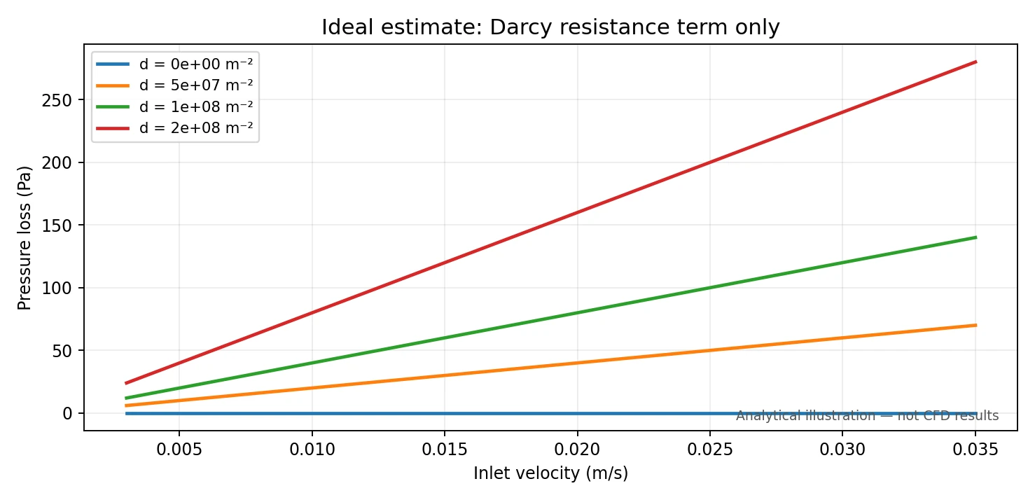
Deep dive · The exact solution of the developed stretch: fully_developed.py
In the W × H rectangular section the equation ν∇²u − νd·u = G with u = 0 on the walls has a double sine series solution; the mean velocity is
and the sum over m is done in closed form with Σm odd 1/(m²+c²) = π tanh(πc/2)/(4c), so the series converges even when the Brinkman layer is thin. With d = 0 one obtains fRe = 76.28 for aspect ratio 0.2, in agreement with the Shah and London polynomial (1978, doi:10.1016/C2013-0-06152-X). The discrete version uses the eigenfunctions of the five-point scheme with the wall at half a cell, sin(mπ(j−½)/N), and gives the solution OpenFOAM would compute on the same section.
#!/usr/bin/env python3
# SPDX-License-Identifier: GPL-3.0-or-later
"""Fully developed laminar flow in the Guide 20 cross-section, empty duct and porous bed.

In the fully developed parts of the channel the 3D problem reduces to the
cross-section equation (kinematic form, f = 0, as in the guide):

    nu*(d2u/dy2 + d2u/dz2) - nu*d*u = G        u = 0 on the four walls

with G = (1/rho) dp/dx. d = 0 gives the empty rectangular duct, d > 0 the
Brinkman-Darcy flow inside the insert. Two solutions are computed:

  exact     double sine series, summed in closed form over one index
  mesh NxM  the same equation discretised as OpenFOAM does on the uniform
            blockMesh grid (cell-centred, Gauss linear uncorrected Laplacian,
            noSlip at half a cell from the centre, porous term per cell),
            solved exactly with a discrete sine expansion; N cells across the
            width (ny) and M across the height (nz)

For every velocity and resistance it prints the pressure gradient [Pa/m], the
ratio to the pure Darcy value mu*d*U (Brinkman wall factor), the Poiseuille
number fRe of the empty duct and the predicted pressure drop between the
x = 35 mm and x = 85 mm sections (10 mm of duct + 40 mm of bed), neglecting
development lengths. It does not run OpenFOAM: it is the a-priori reference
for Exercises A, B and C.

With --k and --void-fraction it also gives the conversion of a first-order
reaction confined to the bed for plug flow (PFR) and for segregated flow
along each streamline of the Brinkman profile (no transverse mixing).

Usage: python3 fully_developed.py [--U 0.0075 0.015 0.03] [--d 0 5e7 1e8 2e8]
                                  [--meshes 10x2 20x4 40x8] [--csv out.csv]
                                  [--k 0.05 --void-fraction 0.7]
"""
import argparse, csv, math, os, sys

W, H = 0.010, 0.002              # channel width (y) and height (z) [m]
L_BED, L_DUCT_35_85 = 0.040, 0.010


def exact_mean(d, nu=1.0):
    """Mean velocity per unit (-G/nu) for the exact series (dimension m^2)."""
    tot = 0.0
    for n in range(1, 40001, 2):
        beta = (n * math.pi / H) ** 2 + d
        c = math.sqrt(beta) * W / math.pi
        x = math.pi * c / 2
        th = 1.0 if x > 20 else math.tanh(x)
        s = (math.pi ** 2 / 8 - math.pi / (4 * c) * th) / c ** 2
        tot += s / n ** 2
    return 64 / math.pi ** 4 * (W ** 2 / math.pi ** 2) * tot


def modes(N, length):
    """Discrete sine modes of the cell-centred operator with walls at the faces."""
    dx = length / N
    out = []
    for m in range(1, N + 1):
        phi = [math.sin(m * math.pi * (j + 0.5) / N) for j in range(N)]
        lam = 4 * math.sin(m * math.pi / (2 * N)) ** 2 / dx ** 2
        out.append((phi, lam, sum(phi), sum(p * p for p in phi)))
    return out


def discrete(ny, nz, d, field=False):
    """Mean velocity per unit (-G/nu) on the ny x nz grid, optionally the cell field."""
    my, mz = modes(ny, W), modes(nz, H)
    tot = 0.0
    coef = []
    for py, ly, sy, ny2 in my:
        row = []
        for pz, lz, sz, nz2 in mz:
            a = (sy * sz) / (ny2 * nz2) / (ly + lz + d)
            row.append(a)
            tot += a * sy * sz
        coef.append(row)
    mean = tot / (ny * nz)
    if not field:
        return mean
    B = [[sum(coef[m][n] * mz[n][0][k] for n in range(nz)) for k in range(nz)] for m in range(ny)]
    u = [[sum(my[m][0][j] * B[m][k] for m in range(ny)) for k in range(nz)] for j in range(ny)]
    return mean, u


def main():
    ap = argparse.ArgumentParser(description=__doc__.split('\n')[0])
    ap.add_argument('--U', type=float, nargs='+', default=[0.0075, 0.015, 0.03])
    ap.add_argument('--d', type=float, nargs='+', default=[0.0, 5e7, 1e8, 2e8])
    ap.add_argument('--meshes', nargs='+', default=['10x2', '20x4', '40x8'])
    ap.add_argument('--nu', type=float, default=1e-6)
    ap.add_argument('--rho', type=float, default=1000.0)
    ap.add_argument('--csv')
    ap.add_argument('--k', type=float)
    ap.add_argument('--void-fraction', type=float, default=0.7)
    a = ap.parse_args()
    if a.csv and os.path.exists(a.csv):
        sys.exit(f'{a.csv} exists: refusing to overwrite')
    meshes = []
    for s in a.meshes:
        ny, nz = (int(v) for v in s.lower().split('x'))
        meshes.append((s, ny, nz))
    mu = a.rho * a.nu
    Dh = 4 * W * H / (2 * (W + H))
    print(f'Cross-section {W*1e3:g} x {H*1e3:g} mm, Dh = {Dh*1e3:.4f} mm, aspect ratio {H/W:g}; nu = {a.nu:g} m2/s, rho = {a.rho:g} kg/m3')
    # mean velocity per unit -G/nu for every d and every grid
    K = {}
    for d in sorted(set([0.0] + a.d)):
        K[('exact', d)] = exact_mean(d)
        for s, ny, nz in meshes:
            K[(s, d)] = discrete(ny, nz, d)
    fRe = 2 * Dh ** 2 / K[('exact', 0.0)]
    print(f'Empty duct, exact: fRe (Darcy friction factor x Re_Dh) = {fRe:.3f}  (Shah & London polynomial: '
          f'{96*(1-1.3553*0.2+1.9467*0.04-1.7012*0.008+0.9564*0.0016-0.2537*0.00032):.3f})')
    for s, ny, nz in meshes:
        print(f'  mesh {s:>6s} (cells {W/ny*1e3:g} x {H/nz*1e3:g} mm): fRe = {2*Dh**2/K[(s, 0.0)]:.3f}  '
              f'({100*(K[("exact", 0.0)]/K[(s, 0.0)]-1):+.2f} % on the duct gradient)')
    print()
    for d in a.d:
        if d <= 0:
            continue
        sk = 1 / math.sqrt(d)
        print(f'd = {d:.3g} 1/m2: K = 1/d = {1/d:.3g} m2, Brinkman length sqrt(K) = {sk*1e3:.4f} mm '
              f'= {sk/(H/max(nz for _, _, nz in meshes)):.2f} of the finest cell height; '
              f'exact Brinkman factor (dp/dx)/(mu d U) = {1/(d*K[("exact", d)]):.4f}')
    print()
    rows = []
    head = f'{"U m/s":>8s} {"d 1/m2":>8s} {"grid":>6s} {"duct Pa/m":>10s} {"bed Pa/m":>11s} {"bed/Darcy":>9s} {"dP35-85 Pa":>10s} {"vs exact":>8s}'
    print(head)
    for U in a.U:
        for d in a.d:
            ref = None
            for s in ['exact'] + [m[0] for m in meshes]:
                g_duct = mu * U / K[(s, 0.0)]
                g_bed = mu * U / K[(s, d)]
                dp = g_duct * L_DUCT_35_85 + g_bed * L_BED
                darcy = mu * d * U
                ref = dp if s == 'exact' else ref
                rows.append(dict(U_m_s=U, d_m_inv2=d, grid=s, duct_Pa_m=g_duct, bed_Pa_m=g_bed,
                                 bed_over_darcy=(g_bed / (darcy / 1.0) if d > 0 else ''), dP_35_85_Pa=dp,
                                 darcy_only_Pa=darcy * L_BED, rel_to_exact=dp / ref - 1))
                print(f'{U:8.4f} {d:8.2g} {s:>6s} {g_duct:10.3f} {g_bed:11.2f} '
                      f'{(g_bed/darcy if d > 0 else float("nan")):9.4f} {dp:10.3f} {100*(dp/ref-1):+7.2f}%')
    if a.k is not None:
        print()
        eps = a.void_fraction
        print(f'First-order reaction in the bed only: k = {a.k:g} 1/s, void fraction {eps:g} (rate eps*k per unit bed volume)')
        print(f'{"U m/s":>8s} {"d 1/m2":>8s} {"X_PFR":>8s} {"X_segregated":>12s}  (200 x 40 grid, Brinkman profile)')
        for d in a.d:
            if d <= 0:
                continue
            mean, u = discrete(200, 40, d, field=True)
            flat = [v / mean for r in u for v in r]          # u/U for every cell
            for U in a.U:
                da = eps * a.k * L_BED / U
                xp = 1 - math.exp(-da)
                xs = sum(f * (1 - math.exp(-da / f)) for f in flat if f > 0) / sum(flat)
                print(f'{U:8.4f} {d:8.2g} {xp:8.5f} {xs:12.5f}')
    if a.csv:
        with open(a.csv, 'x', newline='', encoding='utf-8') as f:
            w = csv.DictWriter(f, fieldnames=list(rows[0]))
            w.writeheader()
            w.writerows(rows)
        print(f'\nwrote {a.csv}')


if __name__ == '__main__':
    main()
Run with the guide values:
$ python3 extra/fully_developed.py --k 0.05 --void-fraction 0.7 --csv fully_developed.csv
Cross-section 10 x 2 mm, Dh = 3.3333 mm, aspect ratio 0.2; nu = 1e-06 m2/s, rho = 1000 kg/m3
Empty duct, exact: fRe (Darcy friction factor x Re_Dh) = 76.282  (Shah & London polynomial: 76.286)
  mesh   10x2 (cells 1 x 1 mm): fRe = 50.246  (-34.13 % on the duct gradient)
  mesh   20x4 (cells 0.5 x 0.5 mm): fRe = 67.315  (-11.75 % on the duct gradient)
  mesh   40x8 (cells 0.25 x 0.25 mm): fRe = 73.799  (-3.26 % on the duct gradient)

d = 5e+07 1/m2: K = 1/d = 2e-08 m2, Brinkman length sqrt(K) = 0.1414 mm = 0.57 of the finest cell height; exact Brinkman factor (dp/dx)/(mu d U) = 1.1970
d = 1e+08 1/m2: K = 1/d = 1e-08 m2, Brinkman length sqrt(K) = 0.1000 mm = 0.40 of the finest cell height; exact Brinkman factor (dp/dx)/(mu d U) = 1.1331
d = 2e+08 1/m2: K = 1/d = 5e-09 m2, Brinkman length sqrt(K) = 0.0707 mm = 0.28 of the finest cell height; exact Brinkman factor (dp/dx)/(mu d U) = 1.0912

   U m/s   d 1/m2   grid  duct Pa/m    bed Pa/m bed/Darcy dP35-85 Pa vs exact
  0.0075        0  exact     25.745       25.75       nan      1.287   +0.00%
  0.0075        0   10x2     16.958       16.96       nan      0.848  -34.13%
  0.0075        0   20x4     22.719       22.72       nan      1.136  -11.75%
  0.0075        0   40x8     24.907       24.91       nan      1.245   -3.26%
  0.0075    5e+07  exact     25.745      448.89    1.1970     18.213   +0.00%
  0.0075    5e+07   10x2     16.958      392.91    1.0478     15.886  -12.78%
  0.0075    5e+07   20x4     22.719      408.42    1.0891     16.564   -9.06%
  0.0075    5e+07   40x8     24.907      427.92    1.1411     17.366   -4.65%
  0.0075    1e+08  exact     25.745      849.81    1.1331     34.250   +0.00%
  0.0075    1e+08   10x2     16.958      767.95    1.0239     30.888   -9.82%
  0.0075    1e+08   20x4     22.719      784.56    1.0461     31.610   -7.71%
  0.0075    1e+08   40x8     24.907      809.64    1.0795     32.635   -4.72%
  0.0075    2e+08  exact     25.745     1636.80    1.0912     65.730   +0.00%
  0.0075    2e+08   10x2     16.958     1517.98    1.0120     60.889   -7.36%
  0.0075    2e+08   20x4     22.719     1535.24    1.0235     61.637   -6.23%
  0.0075    2e+08   40x8     24.907     1564.69    1.0431     62.837   -4.40%
  0.0150        0  exact     51.490       51.49       nan      2.575   +0.00%
  0.0150        0   10x2     33.916       33.92       nan      1.696  -34.13%
  0.0150        0   20x4     45.438       45.44       nan      2.272  -11.75%
  0.0150        0   40x8     49.814       49.81       nan      2.491   -3.26%
  0.0150    5e+07  exact     51.490      897.79    1.1970     36.426   +0.00%
  0.0150    5e+07   10x2     33.916      785.82    1.0478     31.772  -12.78%
  0.0150    5e+07   20x4     45.438      816.84    1.0891     33.128   -9.06%
  0.0150    5e+07   40x8     49.814      855.85    1.1411     34.732   -4.65%
  0.0150    1e+08  exact     51.490     1699.63    1.1331     68.500   +0.00%
  0.0150    1e+08   10x2     33.916     1535.91    1.0239     61.776   -9.82%
  0.0150    1e+08   20x4     45.438     1569.12    1.0461     63.219   -7.71%
  0.0150    1e+08   40x8     49.814     1619.28    1.0795     65.269   -4.72%
  0.0150    2e+08  exact     51.490     3273.61    1.0912    131.459   +0.00%
  0.0150    2e+08   10x2     33.916     3035.95    1.0120    121.777   -7.36%
  0.0150    2e+08   20x4     45.438     3070.47    1.0235    123.273   -6.23%
  0.0150    2e+08   40x8     49.814     3129.39    1.0431    125.674   -4.40%
  0.0300        0  exact    102.981      102.98       nan      5.149   +0.00%
  0.0300        0   10x2     67.833       67.83       nan      3.392  -34.13%
  0.0300        0   20x4     90.875       90.88       nan      4.544  -11.75%
  0.0300        0   40x8     99.628       99.63       nan      4.981   -3.26%
  0.0300    5e+07  exact    102.981     1795.57    1.1970     72.853   +0.00%
  0.0300    5e+07   10x2     67.833     1571.65    1.0478     63.544  -12.78%
  0.0300    5e+07   20x4     90.875     1633.68    1.0891     66.256   -9.06%
  0.0300    5e+07   40x8     99.628     1711.70    1.1411     69.464   -4.65%
  0.0300    1e+08  exact    102.981     3399.25    1.1331    137.000   +0.00%
  0.0300    1e+08   10x2     67.833     3071.82    1.0239    123.551   -9.82%
  0.0300    1e+08   20x4     90.875     3138.24    1.0461    126.438   -7.71%
  0.0300    1e+08   40x8     99.628     3238.56    1.0795    130.539   -4.72%
  0.0300    2e+08  exact    102.981     6547.21    1.0912    262.918   +0.00%
  0.0300    2e+08   10x2     67.833     6071.91    1.0120    243.555   -7.36%
  0.0300    2e+08   20x4     90.875     6140.94    1.0235    246.546   -6.23%
  0.0300    2e+08   40x8     99.628     6258.78    1.0431    251.347   -4.40%

First-order reaction in the bed only: k = 0.05 1/s, void fraction 0.7 (rate eps*k per unit bed volume)
   U m/s   d 1/m2    X_PFR X_segregated  (200 x 40 grid, Brinkman profile)
  0.0075    5e+07  0.17028      0.16732
  0.0150    5e+07  0.08911      0.08822
  0.0300    5e+07  0.04559      0.04535
  0.0075    1e+08  0.17028      0.16842
  0.0150    1e+08  0.08911      0.08857
  0.0300    1e+08  0.04559      0.04545
  0.0075    2e+08  0.17028      0.16922
  0.0150    2e+08  0.08911      0.08880
  0.0300    2e+08  0.04559      0.04551

wrote fully_developed.csv
[exit 0]
The bed/Darcy column is the Brinkman factor: 1.197, 1.133 and 1.091 for the three resistances in the exact solution. In a channel with no-slip walls the exact bed contribution therefore exceeds the guide formula ΔPDarcy = μdLU by 9–20 %, and the difference does not depend on the velocity (it stays linear). The mesh rows show what the computation will return: for Exercise A, with the base mesh, about 63.2 Pa against 68.5 exact and 60 Darcy. The second table compares the PFR conversion with the segregated-flow one along the Brinkman profile (section 14 box).
Practical tip · Separating channel and insert: three estimates to keep distinct in the report
| Quantity | How it is obtained | d = 10⁸, U = 0.015 |
|---|---|---|
| ΔPDarcy (analytical) | μ d Lbed U | 60.0 Pa |
| exact developed ΔP 35–85 mm (analytical) | fully_developed.py, row exact | 68.5 Pa |
| insert contribution (analytical) | ΔP(d) − ΔP(0) | 65.9 Pa = 1.099 × Darcy |
| measured ΔP (CFD, base mesh) | planes at 35 and 85 mm | expected ≈ 63.2 Pa |
| insert contribution (CFD) | ΔP(d) − ΔP(0) at the same velocity | expected ≈ 60.9 Pa = 1.016 × Darcy |
Subtracting the d = 0 case also removes the duct friction over the 40 mm the bed replaces: this is why the insert contribution is smaller than the bed ΔP. In the figures, analytical curves dashed and CFD points filled, with a caption that says so.
14. Chemical conversion: a separate PFR calculation
To connect hydraulic design with chemistry, introduce an explicitly analytical first-order model with assumed bed void fraction ε = 0.70 and constant irreversible rate coefficient k = 0.05 s⁻¹, neglecting axial dispersion and temperature changes:
For U = 0.015 m/s and A = 2×10⁻⁵ m², Q = 3×10⁻⁷ m³/s. With Vbed = 8×10⁻⁷ m³, this yields τ ≈ 1.867 s and X ≈ 8.91% under the assumed ideal PFR model. It is not conversion calculated by OpenFOAM.
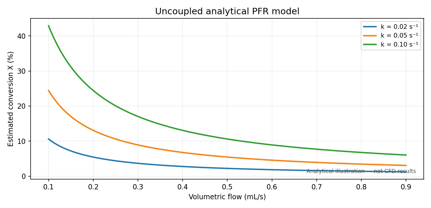
No multiphase transfer, intraparticle diffusion, adsorption, catalytic surface kinetics or thermal feedback is represented in this calculation. A physically reactive CFD case requires independently validated species equations, source terms and appropriate material parameters.
Deep dive · PFR, segregated flow, axial dispersion, CSTR: how much the mixing model matters
The number that governs first-order conversion is Da = εkL/U (bed Damköhler number): 0.187, 0.093 and 0.047 for the three velocities. At small Da all reactor models tend to X ≈ Da, and their differences are of second order in Da. The models to compare:
| Model | Assumption | X, U = 0.0075 | X, U = 0.015 |
|---|---|---|---|
| PFR | plug flow, no axial mixing | 0.1703 | 0.0891 |
| segregated flow (Brinkman, d = 10⁸) | each streamline is a PFR with its own time (Danckwerts 1958, doi:10.1016/0009-2509(58)80040-8; Zwietering 1959, doi:10.1016/0009-2509(59)80068-3) | 0.1684 | 0.0886 |
| axial dispersion, Bo = 32 | Danckwerts conditions (1953, doi:10.1016/0009-2509(53)80001-1), Wehner and Wilhelm solution (1956, doi:10.1016/0009-2509(56)80014-6) | 0.1694 | 0.0889 |
| CSTR | perfect mixing, lower bound | 0.1573 | 0.0854 |
The values come from fully_developed.py --k 0.05 (segregated) and from bed_equivalence.py (dispersion with Pep = 0.5, a typical value for liquids in packed beds: Delgado 2006, doi:10.1007/s00231-005-0019-0). Taylor–Aris dispersion in the empty stretches (Taylor 1953, doi:10.1098/rspa.1953.0139; Aris 1956, doi:10.1098/rspa.1956.0065) does not matter because the reaction only takes place in the bed. The conclusion is clear: at these Da the mixing model shifts X by less than 8 % even in the extreme CSTR case, and by 1 % for realistic segregation and dispersion. The dominant uncertainty is that of k and ε: since X = 1 − exp(−kτ) with τ proportional to ε, a 10 % relative change of k or ε changes X by about 9.5 % at U = 0.015. The assumptions are those of the guide and must be declared as such.
Deep dive · If the reaction took place on the catalyst: Thiele, Weisz–Prater and external transport
The guide treats a homogeneous reaction in the void volume. For a real catalytic support the same overall rate (εk per unit bed volume) corresponds to ks = εk/(1−ε) = 0.117 s⁻¹ per unit particle volume, and two transport resistances can reduce the observed rate. bed_equivalence.py --on-solid estimates them for the equivalent spheres of section 5, with De = 0.1·Dm and Dm = 10⁻⁹ m²/s (liquid):
- internal diffusion: Thiele modulus φ = (dp/6)√(ks/De) = 2.5–5.1, effectiveness factor η = 0.18–0.34 (Thiele 1939, doi:10.1021/ie50355a027); the Weisz–Prater number ηφ² = 2.2–4.7 is larger than 1 (Weisz and Prater 1954, doi:10.1016/S0360-0564(08)60390-9): pore diffusion would control the rate, and a k measured on this bed would be apparent, not intrinsic;
- external transport: with the Wakao and Funazkri correlation (1978, doi:10.1016/0009-2509(78)85120-3) Sh = 25–81 and the ratio between observed rate and kc·a·C is 0.02–0.08, below the 0.15 threshold of the Mears criterion (1971, doi:10.1021/i260040a020): the external film is negligible.
It is an example of why the guide separates result levels so carefully: the k inserted in the PFR (or in the CFD of section 20) must come from a measurement on the same catalyst, at the same particle size, or must include η. The code:
#!/usr/bin/env python3
# SPDX-License-Identifier: GPL-3.0-or-later
"""What physical bed could a Darcy coefficient d represent? Ergun equivalence and reactor regimes.

The guide prescribes d and sets f = 0. Reading d as a packed bed of spheres
of diameter dp and void fraction eps (Ergun 1952, coefficients 150 and 1.75):

    dp/L = 150 mu (1-eps)^2/(eps^3 dp^2) U + 1.75 rho (1-eps)/(eps^3 dp) U^2

so  d = 150 (1-eps)^2/(eps^3 dp^2)  and, in the OpenFOAM form (rho/2) f |U| U,
    f = 3.5 (1-eps)/(eps^3 dp).

For every d > 0 and inlet velocity the script prints the equivalent dp
(Ergun and Kozeny-Carman, 180), the Forchheimer coefficient that the same bed
would have, the ratio of the Forchheimer to the Darcy term neglected by the
guide, the Ergun Reynolds number Re* = U dp/(nu (1-eps)) and the channel-to-particle size ratios
(wall effects). Then, for the analytical first-order reaction of the guide,
it gives the dimensionless groups that tell whether a PFR with the nominal k
is a reasonable model:

  Da = eps k L / U                       Damkoehler number of the bed
  Bo = U L/(eps D_ax)                    axial dispersion (Bodenstein), with
                                         D_ax from Pe_p = U dp/(eps D_ax)
  X for PFR, axial dispersion (Wehner-Wilhelm, closed vessel) and CSTR
  if the reaction were on porous catalyst particles (--on-solid):
  Thiele modulus phi = (dp/6) sqrt(k_s/D_e), effectiveness factor eta,
  Weisz-Prater number eta*phi^2 and the external transfer ratio
  (rate)/(k_c a C) with k_c from Wakao-Funazkri (1978).

All inputs are illustrative defaults of the guide plus declared assumptions
(D_m = 1e-9 m2/s liquid, Pe_p = 0.5, D_e/D_m = 0.1); change them with the options.

Usage: python3 bed_equivalence.py [--d 5e7 1e8 2e8] [--U 0.0075 0.015 0.03]
         [--void-fraction 0.7] [--k 0.05] [--Dm 1e-9] [--Pe-p 0.5]
         [--on-solid --De-ratio 0.1]
"""
import argparse, math

L_BED, W, H = 0.04, 0.010, 0.002


def wehner_wilhelm(Da, Bo):
    a = math.sqrt(1 + 4 * Da / Bo)
    # written with exp(-a Bo/2) factored out to avoid overflow for large Bo
    num = 4 * a * math.exp(Bo / 2 * (1 - a))
    den = (1 + a) ** 2 - (1 - a) ** 2 * math.exp(-a * Bo)
    return 1 - num / den


def main():
    ap = argparse.ArgumentParser(description=__doc__.split('\n')[0])
    ap.add_argument('--d', type=float, nargs='+', default=[5e7, 1e8, 2e8])
    ap.add_argument('--U', type=float, nargs='+', default=[0.0075, 0.015, 0.03])
    ap.add_argument('--void-fraction', type=float, default=0.7)
    ap.add_argument('--k', type=float, default=0.05, help='first-order rate constant per unit fluid volume [1/s]')
    ap.add_argument('--nu', type=float, default=1e-6)
    ap.add_argument('--rho', type=float, default=1000.0)
    ap.add_argument('--Dm', type=float, default=1e-9, help='molecular diffusivity [m2/s]')
    ap.add_argument('--Pe-p', type=float, default=0.5, help='particle Peclet number for axial dispersion')
    ap.add_argument('--on-solid', action='store_true', help='also treat the reaction as occurring inside porous particles')
    ap.add_argument('--De-ratio', type=float, default=0.1, help='effective/molecular diffusivity in the particles')
    a = ap.parse_args()
    e, nu, rho = a.void_fraction, a.nu, a.rho
    mu = rho * nu
    print(f'Assumptions: void fraction {e:g}, nu {nu:g} m2/s, rho {rho:g} kg/m3, k {a.k:g} 1/s, '
          f'D_m {a.Dm:g} m2/s (Sc = {nu/a.Dm:.0f}), Pe_p {a.Pe_p:g}')
    for d in a.d:
        dp = math.sqrt(150 * (1 - e) ** 2 / (e ** 3 * d))
        dp_kc = math.sqrt(180 * (1 - e) ** 2 / (e ** 3 * d))
        f = 3.5 * (1 - e) / (e ** 3 * dp)
        av = 6 * (1 - e) / dp
        print(f'\nd = {d:.3g} 1/m2 -> equivalent spheres dp = {dp*1e3:.3f} mm (Ergun), {dp_kc*1e3:.3f} mm (Kozeny-Carman); '
              f'same bed: f = {f:.4g} 1/m; specific surface a = {av:.4g} 1/m')
        print(f'  channel height / dp = {H/dp:.2f}, width / dp = {W/dp:.2f}, bed length / dp = {L_BED/dp:.1f}'
              + ('  -> fewer than 10 particles across: wall channelling, the uniform-eps model is questionable' if H / dp < 10 else ''))
        print(f'  {"U m/s":>7s} {"Re*":>6s} {"F/D":>6s} {"dP Darcy":>9s} {"dP Ergun":>9s} {"Da":>7s} {"Bo":>7s} {"X_PFR":>7s} {"X_disp":>7s} {"X_CSTR":>7s}')
        for U in a.U:
            rep = U * dp / nu / (1 - e)
            ratio = f * U / (2 * nu * d)
            dpd = mu * d * L_BED * U
            dpe = dpd * (1 + ratio)
            Da = e * a.k * L_BED / U
            Dax = U * dp / (e * a.Pe_p)
            Bo = U * L_BED / (e * Dax)
            xp, xd, xc = 1 - math.exp(-Da), wehner_wilhelm(Da, Bo), Da / (1 + Da)
            print(f'  {U:7.4f} {rep:6.2f} {ratio:6.3f} {dpd:9.3f} {dpe:9.3f} {Da:7.4f} {Bo:7.1f} {xp:7.4f} {xd:7.4f} {xc:7.4f}')
        if a.on_solid:
            De = a.De_ratio * a.Dm
            ks = e * a.k / (1 - e)                       # same overall rate, referred to particle volume
            phi = dp / 6 * math.sqrt(ks / De)
            eta = (1 / math.tanh(3 * phi) - 1 / (3 * phi)) / phi
            print(f'  reaction inside the particles: k_s = {ks:.4g} 1/s, D_e = {De:.3g} m2/s, Thiele phi = {phi:.3f}, '
                  f'eta = {eta:.3f}, Weisz-Prater eta*phi^2 = {eta*phi**2:.3f} ' + ('(> 1: internal diffusion controls)' if eta * phi ** 2 > 1 else '(< 0.3: kinetic regime)' if eta * phi ** 2 < 0.3 else '(intermediate)'))
            for U in a.U:
                rep0 = U * dp / nu
                Sh = 2 + 1.1 * (nu / a.Dm) ** (1 / 3) * rep0 ** 0.6
                kc = Sh * a.Dm / dp
                ext = eta * ks * (1 - e) / (kc * av)
                print(f'    U = {U:.4f}: Re = {rep0:.2f}, Sh = {Sh:.2f}, k_c = {kc:.3g} m/s, observed rate/(k_c a C) = {ext:.3f}'
                      + ('  (< 0.15: external transfer negligible)' if ext < 0.15 else '  (external transfer matters)'))


if __name__ == '__main__':
    main()
Practical tip · τ, interstitial velocity and sensitivity of the conversion
- τ = εVbed/Q is the mean time in the void volume: it equals L/(U/ε), with U/ε = 0.0214 m/s the mean interstitial velocity for U = 0.015;
analyze_measurements.pyuses the measured Qin, not A·U: a flow-rate error passes straight to τ, one more reason to measure the flow rate withphi;- dX/dk = τ e−kτ: at U = 0.015 an error of 0.005 s⁻¹ on k (10 %) shifts X by 0.0085 out of 0.089;
- Vbed is fixed in the script at 8·10⁻⁷ m³: if the zone changes (or a mesh does not align faces with 40 and 80 mm) the volume must be corrected;
case_estimates.pyrecomputes it from the cells.
15. Exercise A — Reference hydraulic case
Run the case with inlet speed 0.015 m/s and d = 10⁸ m⁻². Inspect checkMesh, the number of cells in the selected zone, residuals and flow balance. Export one central velocity profile, a pressure map and the two measurement cross-sections. Prepare a table of ΔP, Q and the time window used for assessing stabilization.
Completion standard: no final number should be reported without a log, measurement location and a defensible stabilization criterion.
Practical tip · Exercise A step by step, with the expected values
cd ~/OpenFOAM/guide20
source /opt/OpenFOAM-14/etc/bashrc
python3 exercises/prepare_campaign.py --out ~/OpenFOAM/guide20/exA --quick
python3 extra/case_estimates.py exA/U0.0150_D1e08
python3 extra/add_monitors.py exA/U*
bash extra/run_case_checked.sh "$HOME/OpenFOAM/guide20/exA/U0.0150_D1e08"
python3 extra/extract_measurements.py exA --cases U0.0150_D1e08 --out exA_measurements.csv --evidence exA_evidence.csv
python3 exercises/analyze_measurements.py --measurements exA_measurements.csv --out exA_results.csv| Check | Expected value | Where to read it |
|---|---|---|
| cells; zone cells | 7680; 2560 | log.checkMesh; print generator |
| area and faces of the planes | 2.0·10⁻⁵ m²; 80 | postProcessing/pUp/0/surfaceFieldValue.dat |
| inlet flow rate | 3.0·10⁻⁷ m³/s | q_in_vs_AU ≈ 0 |
| flow balance | < 10⁻⁴ (with phi) | flow_balance |
| duct gradient | ≈ 45 Pa/m (mesh), 51.5 exact | grad_duct_Pa_m |
| bed gradient | ≈ 1570 Pa/m (mesh), 1700 exact, 1500 Darcy | grad_bed_Pa_m |
| ΔP between 35 and 85 mm | ≈ 63 Pa (mesh), 68.5 exact, 60 Darcy | delta_p_measured_Pa |
| velocity on the axis | ≈ 1.5 U in the duct, ≈ 1.04 U in the bed (mesh); 1.72 and 1.13 exact | centreline, profileBed |
| drift in the final window | < 10⁻⁴ | drift_dP |
A deviation larger than 2–3 % from the “mesh” values indicates a set-up error (zone, d, viscosity, flow rate), not a discretisation problem: the mesh predictions are computed with the same scheme as the solver. The completion criterion of the guide asks for the log, the measurement coordinates and the stability criterion: they are all in the RUN_*, log.* and exA_evidence.csv files.
16. Exercise B — Flow-rate and resistance sweep
Prepare the 12 cases. At fixed speed compare d = 0, 5×10⁷, 10⁸ and 2×10⁸ m⁻². At fixed d compare the three inlet speeds. Plot ΔP versus U and clearly identify CFD-measured points versus analytical predictions. Discuss whether the pressure response appears linear over the sampled range, and account for duct losses.
Compare only cases with comparable numerical quality. If a case is persistently oscillatory, report this rather than silently forcing its last saved pressure into a fitted line.
Practical tip · campaign_fit.py: ΔP(U) regressions, insert contribution and apparent permeability
The script joins the measurements file and the results file of analyze_measurements.py, excludes the rows with a CHECK balance and, for every d, computes the line through the origin and the one with intercept, then the insert contribution ΔP(d) − ΔP(0) at equal velocity, its ratio to μdLU and the apparent permeability Kapp = μLU/ΔPins. The optional plot draws the CFD points filled and the Darcy lines dashed, distinguished in the legend.
#!/usr/bin/env python3
# SPDX-License-Identifier: GPL-3.0-or-later
"""Exercise B: dP(U) fits, insert contribution and apparent permeability from the measured campaign.

Joins the measurements file (the input of analyze_measurements.py, which has
velocity and d of every case) with its results file (delta_p_measured_Pa) and,
for every Darcy coefficient d:

  * fits dP = a*U through the origin and dP = a*U + b, with R^2 and the
    largest relative residual: in the Darcy regime with f = 0 the CFD pressure
    drop must be proportional to U (inertia only adds small terms in the
    development regions);
  * subtracts the d = 0 control at the same velocity: dP_insert = dP(d) - dP(0),
    the additional loss caused by the insert between the two planes;
  * compares dP_insert with the Darcy-only estimate mu*d*L*U and gives the
    apparent permeability K_app = mu*L*U/dP_insert and the ratio K_app*d
    (1 = pure Darcy; < 1 when wall friction in the bed, i.e. the Brinkman
    layer, adds to the Darcy resistance).

Rows whose flow_balance_status is CHECK are reported and excluded from the
fits. Optional: --out CSV of the table, --plot PNG (matplotlib) with measured
points (CFD) and the Darcy-only lines (analytical) drawn distinctly.

Usage: python3 campaign_fit.py --measurements misure_reali.csv --results risultati_calcolati.csv
                               [--out fit.csv] [--plot dP_U.png] [--L 0.04]
"""
import argparse, csv, math, os, sys


def fit0(pts):
    sxx = sum(u * u for u, _ in pts)
    a = sum(u * p for u, p in pts) / sxx
    return a


def fit1(pts):
    n = len(pts)
    mu_ = sum(u for u, _ in pts) / n
    mp = sum(p for _, p in pts) / n
    sxx = sum((u - mu_) ** 2 for u, _ in pts)
    a = sum((u - mu_) * (p - mp) for u, p in pts) / sxx
    return a, mp - a * mu_


def r2(pts, f):
    mp = sum(p for _, p in pts) / len(pts)
    ss = sum((p - mp) ** 2 for _, p in pts)
    return 1 - sum((p - f(u)) ** 2 for u, p in pts) / ss if ss else float('nan')


def main():
    ap = argparse.ArgumentParser(description=__doc__.split('\n')[0])
    ap.add_argument('--measurements', required=True)
    ap.add_argument('--results', required=True)
    ap.add_argument('--out')
    ap.add_argument('--plot')
    ap.add_argument('--L', type=float, default=0.04, help='bed length [m]')
    a = ap.parse_args()
    for p in (a.out, a.plot):
        if p and os.path.exists(p):
            sys.exit(f'{p} exists: refusing to overwrite')
    M = {r['case_id']: r for r in csv.DictReader(open(a.measurements, newline='', encoding='utf-8-sig'))}
    R = list(csv.DictReader(open(a.results, newline='', encoding='utf-8-sig')))
    data = {}
    for r in R:
        m = M.get(r['case_id'])
        if m is None:
            sys.exit(f'{r["case_id"]} is in the results but not in the measurements file')
        if r.get('flow_balance_status') == 'CHECK':
            print(f'{r["case_id"]}: flow balance CHECK ({r["flow_balance_relative"]}): excluded')
            continue
        U, d = float(m['velocity_in_m_s']), float(m['d_m_inv2'])
        mu = float(m['rho_kg_m3']) * float(m['nu_m2_s'])
        data.setdefault(d, []).append((U, float(r['delta_p_measured_Pa']), mu, r['case_id']))
    if not data:
        sys.exit('no usable rows')
    base = {round(U, 9): p for U, p, _, _ in data.get(0.0, [])}
    rows = []
    print(f'{"d 1/m2":>8s} {"n":>2s} {"a Pa.s/m":>10s} {"R2(0)":>8s} {"max res":>8s} {"b Pa":>9s} {"b/dPmax":>8s}')
    for d in sorted(data):
        pts = sorted((U, p) for U, p, _, _ in data[d])
        if len(pts) >= 2:
            a0 = fit0(pts)
            res = max(abs(p - a0 * U) / abs(p) for U, p in pts if p)
            a1, b1 = fit1(pts) if len(pts) >= 3 else (float('nan'), float('nan'))
            print(f'{d:8.3g} {len(pts):2d} {a0:10.5g} {r2(pts, lambda u: a0*u):8.5f} {res:8.3g} {b1:9.3g} {b1/max(p for _, p in pts):8.3g}')
        for U, p, mu, cid in sorted(data[d]):
            darcy = mu * d * a.L * U
            row = dict(case_id=cid, U_m_s=U, d_m_inv2=d, dP_measured_Pa=p, darcy_only_Pa=darcy)
            b = base.get(round(U, 9))
            if d > 0 and b is not None:
                ins = p - b
                row.update(dP_control_Pa=b, dP_insert_Pa=ins, insert_over_darcy=ins / darcy,
                           K_app_m2=mu * a.L * U / ins if ins > 0 else float('nan'))
                row['K_app_times_d'] = row['K_app_m2'] * d
            rows.append(row)
    print()
    print(f'{"case":16s} {"dP Pa":>9s} {"control":>8s} {"insert":>9s} {"Darcy":>9s} {"ins/Darcy":>9s} {"K_app m2":>10s} {"K_app*d":>8s}')
    for r in rows:
        if 'dP_insert_Pa' in r:
            print(f'{r["case_id"]:16s} {r["dP_measured_Pa"]:9.4g} {r["dP_control_Pa"]:8.4g} {r["dP_insert_Pa"]:9.4g} {r["darcy_only_Pa"]:9.4g} '
                  f'{r["insert_over_darcy"]:9.4f} {r["K_app_m2"]:10.4g} {r["K_app_times_d"]:8.4f}')
        elif r['d_m_inv2'] == 0:
            print(f'{r["case_id"]:16s} {r["dP_measured_Pa"]:9.4g}  (control, d = 0)')
        else:
            print(f'{r["case_id"]:16s} {r["dP_measured_Pa"]:9.4g}  (no d = 0 control at this velocity)')
    if a.out:
        keys = []
        for r in rows:
            keys += [k for k in r if k not in keys]
        with open(a.out, 'x', newline='', encoding='utf-8') as f:
            w = csv.DictWriter(f, fieldnames=keys)
            w.writeheader()
            w.writerows(rows)
        print(f'\nwrote {a.out}')
    if a.plot:
        import matplotlib
        matplotlib.use('Agg')
        import matplotlib.pyplot as plt
        fig, ax = plt.subplots(figsize=(7, 4.5))
        for d in sorted(data):
            pts = sorted((U, p) for U, p, _, _ in data[d])
            l, = ax.plot([u for u, _ in pts], [p for _, p in pts], 'o-', label=f'CFD measured, d = {d:.3g} 1/m2')
            if d > 0:
                mu = data[d][0][2]
                us = [0, max(u for u, _ in pts)]
                ax.plot(us, [mu * d * a.L * u for u in us], '--', color=l.get_color(), lw=1, label=f'Darcy only (analytical), d = {d:.3g}')
        ax.set_xlabel('inlet velocity U [m/s]')
        ax.set_ylabel('dP between the two planes [Pa]')
        ax.grid(alpha=0.3)
        ax.legend(fontsize=7)
        fig.tight_layout()
        fig.savefig(a.plot, dpi=150)
        print(f'wrote {a.plot}')


if __name__ == '__main__':
    main()
Test with the OpenFOAM commands replaced by placeholders (blockMesh, checkMesh, createZones and foamRun that only create the expected files; the postProcessing files are written by extra/make_synthetic_monitors.py and tagged SYNTHETIC: they serve to test the scripts, they are not CFD results). Paths shortened to /home/user.
$ python3 exercises/analyze_measurements.py --measurements run01_measurements.csv --out run01_results.csv
Wrote 12 measured rows to run01_results.csv
[exit 0]
$ python3 extra/campaign_fit.py --measurements run01_measurements.csv --results run01_results.csv --out run01_fit.csv --plot run01_dP_U.png
  d 1/m2  n   a Pa.s/m    R2(0)  max res      b Pa  b/dPmax
       0  3     151.46  1.00000 2.52e-09         0        0
   5e+07  3     2208.5  1.00000 1.15e-09     5e-08 7.55e-10
   1e+08  3     4214.6  1.00000 2.71e-09   1.5e-07 1.19e-09
   2e+08  3     8218.2  1.00000 3.24e-09     3e-07 1.22e-09

case                 dP Pa  control    insert     Darcy ins/Darcy   K_app m2  K_app*d
U0.0075_D0e00        1.136  (control, d = 0)
U0.0150_D0e00        2.272  (control, d = 0)
U0.0300_D0e00        4.544  (control, d = 0)
U0.0075_D5e07        16.56    1.136     15.43        15    1.0285  1.945e-08   0.9723
U0.0150_D5e07        33.13    2.272     30.86        30    1.0285  1.945e-08   0.9723
U0.0300_D5e07        66.26    4.544     61.71        60    1.0285  1.945e-08   0.9723
U0.0075_D1e08        31.61    1.136     30.47        30    1.0158  9.845e-09   0.9845
U0.0150_D1e08        63.22    2.272     60.95        60    1.0158  9.845e-09   0.9845
U0.0300_D1e08        126.4    4.544     121.9       120    1.0158  9.845e-09   0.9845
U0.0075_D2e08        61.64    1.136      60.5        60    1.0083  4.959e-09   0.9917
U0.0150_D2e08        123.3    2.272       121       120    1.0083  4.959e-09   0.9917
U0.0300_D2e08        246.5    4.544       242       240    1.0083  4.959e-09   0.9917

wrote run01_fit.csv
wrote run01_dP_U.png
[exit 0]
Deep dive · How to read the regression: linearity, intercept and apparent K
- with f = 0 and laminar flow the equations are linear in U apart from convection, which acts only in the development stretches: the maximum residual of the line through the origin must be below 1 %. A systematic curvature (positive residuals at the ends, negative in the middle) points to inertia in the transition zones or to non-steady cases;
- an intercept b different from zero beyond 1 % of the largest ΔP has no physical meaning in this model: look for a different pressure reference between cases or a conversion error;
- the ratio Kapp·d is 1 for pure Darcy; in the exact solution it is 1/1.099 = 0.91 for d = 10⁸ (wall friction in the bed minus friction of the replaced duct), on the base mesh about 0.98. The measured value tells how much of the wall friction the mesh captures;
- with a real medium (f > 0) the slope of ΔP/U against U gives f, as in the permeability test of section 5: the same analysis becomes a calibration.
17. Exercise C — Grid sensitivity and uncertainty
Repeat at least the central case using 48×10×2, 96×20×4 and 192×40×8 cells by modifying nx, ny, nz in fresh copies of blockMeshDict. Keep the physical geometry, viscosity, d and boundary conditions identical. Record the rising computational cost of fine meshes.
Compare ΔP on the same fixed cross-sections and inspect mass balance. Reproducibility of a single run is not mesh independence: choose a justified tolerance, examine refinement trends and, if appropriate, use the GCI methodology covered in Guide 4.
Practical tip · prepare_mesh_series.py and gci.py: the three meshes and the convergence index
prepare_mesh_series.py copies a never-run case into three new folders changing only the nx ny nz macros (factors 0.5, 1, 2) and checks that the planes at 35, 40, 80 and 85 mm stay on cell faces. gci.py applies the Celik et al. procedure (2008, doi:10.1115/1.2960953): apparent order with iteration for non-constant ratios, extrapolated value, relative errors, GCI and asymptotic-range check; it reports oscillatory convergence and differences that grow with refinement instead of hiding them.
#!/usr/bin/env python3
# SPDX-License-Identifier: GPL-3.0-or-later
"""Exercise C: copies of one fresh reactor case on refined and coarsened meshes.

Copies CASE (never run: no logs, no mesh) into new directories next to a
--out folder, one per scale factor, changing only the nx, ny, nz macros of
system/blockMeshDict (default factors 0.5, 1, 2: 48x10x2, 96x20x4, 192x40x8
for the template). Geometry, viscosity, d, boundary conditions and controls
are untouched; the x positions 35, 40, 80 and 85 mm stay on cell faces for
these factors (checked). Writes mesh_series.csv with the cells and the
nominal spacing h = (V/N)^(1/3) needed by gci.py. Nothing existing is
overwritten.

Usage: python3 prepare_mesh_series.py CASE --out SERIES_DIR [--factors 0.5 1 2]
"""
import argparse, csv, glob, os, re, shutil, sys


def main():
    ap = argparse.ArgumentParser(description=__doc__.split('\n')[0])
    ap.add_argument('case')
    ap.add_argument('--out', required=True)
    ap.add_argument('--factors', type=float, nargs='+', default=[0.5, 1.0, 2.0])
    a = ap.parse_args()
    if os.path.exists(a.out):
        sys.exit(f'{a.out} exists: refusing to overwrite')
    bad = glob.glob(os.path.join(a.case, 'log.*')) + [p for p in (os.path.join(a.case, 'constant', 'polyMesh'), os.path.join(a.case, 'postProcessing')) if os.path.exists(p)]
    if bad:
        sys.exit(f'{a.case} has already been meshed or run ({", ".join(os.path.basename(b) for b in bad)}): start from a fresh copy')
    bm = open(os.path.join(a.case, 'system', 'blockMeshDict'), encoding='utf-8').read()
    n0 = {}
    for k in ('nx', 'ny', 'nz'):
        m = re.findall(r'(?m)^' + k + r'\s+(\d+)\s*;', bm)
        if len(m) != 1:
            sys.exit(f'{k} macro not found exactly once in blockMeshDict')
        n0[k] = int(m[0])
    xs = [float(v) for v in re.findall(r'\(\s*([-+0-9.eE]+)\s+[-+0-9.eE]+\s+[-+0-9.eE]+\s*\)', bm.split('blocks')[0])]
    ys = [float(v) for v in re.findall(r'\(\s*[-+0-9.eE]+\s+([-+0-9.eE]+)\s+[-+0-9.eE]+\s*\)', bm.split('blocks')[0])]
    zs = [float(v) for v in re.findall(r'\(\s*[-+0-9.eE]+\s+[-+0-9.eE]+\s+([-+0-9.eE]+)\s*\)', bm.split('blocks')[0])]
    L, V = max(xs) - min(xs), (max(xs) - min(xs)) * (max(ys) - min(ys)) * (max(zs) - min(zs))
    rows = []
    plan = []
    for f in a.factors:
        n = {k: v * f for k, v in n0.items()}
        if any(abs(v - round(v)) > 1e-9 or round(v) < 1 for v in n.values()):
            sys.exit(f'factor {f:g} gives non-integer cell numbers {n}')
        n = {k: int(round(v)) for k, v in n.items()}
        dx = L / n['nx']
        for x in (0.035, 0.040, 0.080, 0.085):
            if abs(x / dx - round(x / dx)) > 1e-6:
                sys.exit(f'factor {f:g}: x = {x*1e3:g} mm is not on a cell face (dx = {dx*1e3:g} mm)')
        plan.append((f, n))
    os.makedirs(a.out)
    for f, n in plan:
        name = f'{os.path.basename(os.path.normpath(a.case))}_m{n["nx"]}x{n["ny"]}x{n["nz"]}'
        dst = os.path.join(a.out, name)
        shutil.copytree(a.case, dst)
        t = bm
        for k, v in n.items():
            t = re.sub(r'(?m)^(' + k + r'\s+)\d+(\s*;)', lambda m: f'{m.group(1)}{v}{m.group(2)}', t)
        open(os.path.join(dst, 'system', 'blockMeshDict'), 'w', encoding='utf-8', newline='\n').write(t)
        N = n['nx'] * n['ny'] * n['nz']
        h = (V / N) ** (1 / 3)
        rows.append(dict(case_id=name, factor=f'{f:g}', nx=n['nx'], ny=n['ny'], nz=n['nz'], cells=N, h_m=f'{h:.6g}'))
        print(f'{dst}: {n["nx"]} x {n["ny"]} x {n["nz"]} = {N} cells, h = {h*1e3:.4g} mm')
    with open(os.path.join(a.out, 'mesh_series.csv'), 'x', newline='', encoding='utf-8') as fo:
        w = csv.DictWriter(fo, fieldnames=list(rows[0]))
        w.writeheader()
        w.writerows(rows)


if __name__ == '__main__':
    main()
#!/usr/bin/env python3
# SPDX-License-Identifier: GPL-3.0-or-later
"""Grid Convergence Index of one observable on three meshes (Celik et al. 2008, ASME JFE procedure).
Give the observable on the fine, medium and coarse mesh (in this order) and the
number of cells of each mesh (3D: h = (V/N)^(1/3)) or the refinement ratios.
The script computes the apparent order p (fixed-point iteration for
non-constant ratios), the Richardson extrapolated value, the approximate and
extrapolated relative errors, GCI_fine and GCI_medium, and the asymptotic
range check GCI_medium / (r21^p GCI_fine), which must be close to 1.
Oscillatory convergence (the two differences of opposite sign) and
differences that grow under refinement (apparent order <= 0: the meshes are
not in the asymptotic range) are reported instead of hidden.
Usage: python3 gci.py --values 65.27 63.22 61.78 --cells 61440 7680 960
python3 gci.py --values f1 f2 f3 --ratios 2 2 [--Fs 1.25]
"""
import argparse, math, sys
def main():
ap = argparse.ArgumentParser(description=__doc__.split('\n')[0])
ap.add_argument('--values', type=float, nargs=3, required=True, metavar=('FINE', 'MEDIUM', 'COARSE'))
g = ap.add_mutually_exclusive_group(required=True)
g.add_argument('--cells', type=float, nargs=3, metavar=('N1', 'N2', 'N3'))
g.add_argument('--ratios', type=float, nargs=2, metavar=('R21', 'R32'))
ap.add_argument('--Fs', type=float, default=1.25, help='safety factor (1.25 for three meshes)')
a = ap.parse_args()
f1, f2, f3 = a.values
if a.cells:
n1, n2, n3 = a.cells
r21, r32 = (n1 / n2) ** (1 / 3), (n2 / n3) ** (1 / 3)
else:
r21, r32 = a.ratios
if r21 <= 1 or r32 <= 1:
sys.exit('refinement ratios must be > 1 (order: fine, medium, coarse)')
e21, e32 = f2 - f1, f3 - f2
print(f'values: fine {f1:g}, medium {f2:g}, coarse {f3:g}; r21 = {r21:.4g}, r32 = {r32:.4g}')
print(f'differences: e21 = f2 - f1 = {e21:.6g}, e32 = f3 - f2 = {e32:.6g}')
if e21 == 0 or e32 == 0:
sys.exit('a difference is zero: the observable does not change with the mesh at this precision')
s = math.copysign(1.0, e32 / e21)
if s < 0:
print('OSCILLATORY convergence (differences of opposite sign): the apparent order below is only indicative')
p = abs(math.log(abs(e32 / e21))) / math.log(r21)
for _ in range(200):
q = math.log((r21 ** p - s) / (r32 ** p - s))
pn = abs(math.log(abs(e32 / e21)) + q) / math.log(r21)
if abs(pn - p) < 1e-10:
break
p = pn
if abs(e32) < abs(e21):
print(f'the difference GROWS under refinement (|e32| < |e21|): not in the asymptotic range, '
f'p = {p:.3f} is meaningless and no error band is given; refine further')
return
fext = (r21 ** p * f1 - f2) / (r21 ** p - 1)
ea21 = abs((f1 - f2) / f1)
eext21 = abs((fext - f1) / fext)
gci21 = a.Fs * ea21 / (r21 ** p - 1)
gci32 = a.Fs * abs((f2 - f3) / f2) / (r32 ** p - 1)
print(f'apparent order p = {p:.4f}')
print(f'extrapolated value = {fext:.6g}')
print(f'approximate relative error e_a21 = {100*ea21:.3f} %, extrapolated relative error e_ext21 = {100*eext21:.3f} %')
print(f'GCI_fine = {100*gci21:.3f} % -> {f1:.6g} +/- {gci21*abs(f1):.3g}')
print(f'GCI_medium = {100*gci32:.3f} %; asymptotic range check GCI_medium/(r21^p GCI_fine) = {gci32/(r21**p*gci21):.4f} (should be about 1)')
if __name__ == '__main__':
main()Test with the OpenFOAM commands replaced by placeholders (blockMesh, checkMesh, createZones and foamRun that only create the expected files; the postProcessing files are written by extra/make_synthetic_monitors.py and tagged SYNTHETIC: they serve to test the scripts, they are not CFD results). Paths shortened to /home/user.
$ python3 exercises/prepare_campaign.py --out ~/OpenFOAM/guide20/ref02 --quick
Created 3 independent cases at /home/user/OpenFOAM/guide20/ref02
[exit 0]
$ python3 extra/prepare_mesh_series.py ref02/U0.0150_D1e08 --out ~/OpenFOAM/guide20/meshC
/home/user/OpenFOAM/guide20/meshC/U0.0150_D1e08_m48x10x2: 48 x 10 x 2 = 960 cells, h = 1.357 mm
/home/user/OpenFOAM/guide20/meshC/U0.0150_D1e08_m96x20x4: 96 x 20 x 4 = 7680 cells, h = 0.6786 mm
/home/user/OpenFOAM/guide20/meshC/U0.0150_D1e08_m192x40x8: 192 x 40 x 8 = 61440 cells, h = 0.3393 mm
[exit 0]
$ cat meshC/mesh_series.csv
case_id,factor,nx,ny,nz,cells,h_m
U0.0150_D1e08_m48x10x2,0.5,48,10,2,960,0.00135721
U0.0150_D1e08_m96x20x4,1,96,20,4,7680,0.000678604
U0.0150_D1e08_m192x40x8,2,192,40,8,61440,0.000339302
[exit 0]
$ diff ref02/U0.0150_D1e08/system/blockMeshDict meshC/U0.0150_D1e08_m192x40x8/system/blockMeshDict
10,12c10,12
< nx 96;
< ny 20;
< nz 4;
---
> nx 192;
> ny 40;
> nz 8;
[exit 1]
$ python3 extra/add_monitors.py meshC/U0.0150_D1e08_m*
meshC/U0.0150_D1e08_m192x40x8: system/functions written (monitors at x = 0.035, 0.06, 0.085 m)
meshC/U0.0150_D1e08_m48x10x2: system/functions written (monitors at x = 0.035, 0.06, 0.085 m)
meshC/U0.0150_D1e08_m96x20x4: system/functions written (monitors at x = 0.035, 0.06, 0.085 m)
[exit 0]
$ for c in meshC/U0.0150_D1e08_m*; do bash extra/run_case_checked.sh "$(pwd)/$c" || break; done
Completed: /home/user/OpenFOAM/guide20/meshC/U0.0150_D1e08_m192x40x8
Completed: /home/user/OpenFOAM/guide20/meshC/U0.0150_D1e08_m48x10x2
Completed: /home/user/OpenFOAM/guide20/meshC/U0.0150_D1e08_m96x20x4
[exit 0]
$ python3 extra/extract_measurements.py meshC --cases U0.0150_D1e08_m192x40x8 U0.0150_D1e08_m96x20x4 U0.0150_D1e08_m48x10x2 --out meshC_measurements.csv --evidence meshC_evidence.csv
U0.0150_D1e08_m192x40x8: dP = 65.2693 Pa, drift -8.97e-07, balance 1.41e-07, Q_in/(A U)-1 = -2.22e-16, bed gradient 1619.28 Pa/m
U0.0150_D1e08_m96x20x4: dP = 63.2193 Pa, drift -8.96e-07, balance 1.41e-07, Q_in/(A U)-1 = -2.22e-16, bed gradient 1569.12 Pa/m
U0.0150_D1e08_m48x10x2: dP = 61.7755 Pa, drift -8.9e-07, balance 1.41e-07, Q_in/(A U)-1 = -2.22e-16, bed gradient 1535.91 Pa/m
wrote meshC_measurements.csv (3 cases) and meshC_evidence.csv
[exit 0]
$ python3 extra/gci.py --values 65.2693 63.2193 61.7755 --cells 61440 7680 960
values: fine 65.2693, medium 63.2193, coarse 61.7755; r21 = 2, r32 = 2
differences: e21 = f2 - f1 = -2.05, e32 = f3 - f2 = -1.4438
the difference GROWS under refinement (|e32| < |e21|): not in the asymptotic range, p = 0.506 is meaningless and no error band is given; refine further
[exit 0]
$ python3 extra/fully_developed.py --U 0.015 --d 0 1e8 --meshes 10x2 20x4 40x8 80x16 160x32 320x64
Cross-section 10 x 2 mm, Dh = 3.3333 mm, aspect ratio 0.2; nu = 1e-06 m2/s, rho = 1000 kg/m3
Empty duct, exact: fRe (Darcy friction factor x Re_Dh) = 76.282  (Shah & London polynomial: 76.286)
  mesh   10x2 (cells 1 x 1 mm): fRe = 50.246  (-34.13 % on the duct gradient)
  mesh   20x4 (cells 0.5 x 0.5 mm): fRe = 67.315  (-11.75 % on the duct gradient)
  mesh   40x8 (cells 0.25 x 0.25 mm): fRe = 73.799  (-3.26 % on the duct gradient)
  mesh  80x16 (cells 0.125 x 0.125 mm): fRe = 75.643  (-0.84 % on the duct gradient)
  mesh 160x32 (cells 0.0625 x 0.0625 mm): fRe = 76.121  (-0.21 % on the duct gradient)
  mesh 320x64 (cells 0.03125 x 0.03125 mm): fRe = 76.242  (-0.05 % on the duct gradient)

d = 1e+08 1/m2: K = 1/d = 1e-08 m2, Brinkman length sqrt(K) = 0.1000 mm = 3.20 of the finest cell height; exact Brinkman factor (dp/dx)/(mu d U) = 1.1331

   U m/s   d 1/m2   grid  duct Pa/m    bed Pa/m bed/Darcy dP35-85 Pa vs exact
  0.0150        0  exact     51.490       51.49       nan      2.575   +0.00%
  0.0150        0   10x2     33.916       33.92       nan      1.696  -34.13%
  0.0150        0   20x4     45.438       45.44       nan      2.272  -11.75%
  0.0150        0   40x8     49.814       49.81       nan      2.491   -3.26%
  0.0150        0  80x16     51.059       51.06       nan      2.553   -0.84%
  0.0150        0 160x32     51.382       51.38       nan      2.569   -0.21%
  0.0150        0 320x64     51.463       51.46       nan      2.573   -0.05%
  0.0150    1e+08  exact     51.490     1699.63    1.1331     68.500   +0.00%
  0.0150    1e+08   10x2     33.916     1535.91    1.0239     61.776   -9.82%
  0.0150    1e+08   20x4     45.438     1569.12    1.0461     63.219   -7.71%
  0.0150    1e+08   40x8     49.814     1619.28    1.0795     65.269   -4.72%
  0.0150    1e+08  80x16     51.059     1666.07    1.1107     67.154   -1.97%
  0.0150    1e+08 160x32     51.382     1689.41    1.1263     68.090   -0.60%
  0.0150    1e+08 320x64     51.463     1696.92    1.1313     68.392   -0.16%
[exit 0]
$ python3 extra/gci.py --values 68.090 67.154 65.269 --cells 3932160 491520 61440
values: fine 68.09, medium 67.154, coarse 65.269; r21 = 2, r32 = 2
differences: e21 = f2 - f1 = -0.936, e32 = f3 - f2 = -1.885
apparent order p = 1.0100
extrapolated value = 69.0132
approximate relative error e_a21 = 1.375 %, extrapolated relative error e_ext21 = 1.338 %
GCI_fine = 1.695 %  ->  68.09 +/- 1.15
GCI_medium = 3.461 %; asymptotic range check GCI_medium/(r21^p GCI_fine) = 1.0139 (should be about 1)
[exit 0]
Deep dive · Why the GCI does not work with 48×10×2, 96×20×4 and 192×40×8, and how to fix it
The fully_developed.py predictions for ΔP between the planes (d = 10⁸, U = 0.015) are 61.8, 63.2 and 65.3 Pa: the difference between medium and fine mesh (2.05 Pa) is larger than between coarse and medium (1.44 Pa). The observable is not in the asymptotic range, and gci.py says so instead of producing an error band. The cause is the Brinkman layer: as long as the wall cells are larger than √K = 0.1 mm, refining adds friction that was not there before. Continuing with uniform meshes (40×8 → 80×16 → 160×32 in the section) the apparent order only rises to 1.0 and the extrapolated estimate (69.0 Pa) exceeds the exact value (68.5); the GCI band of ±1.15 Pa contains it, but at the cost of almost four million cells.
The remedy is a mesh graded towards the walls, with the first cell thinner than √K. In blockMeshDict multi-section grading is enough (length fraction, cell fraction, expansion ratio); for example, with nx 96; ny 40; nz 16;:
blocks
(
    hex (0 1 2 3 4 5 6 7) ($nx $ny $nz)
    simpleGrading
    (
        1
        ((0.1 0.25 4) (0.8 0.5 1) (0.1 0.25 0.25))
        ((0.25 0.375 4) (0.5 0.25 1) (0.25 0.375 0.25))
    )
);
In y: 10 cells in the first millimetre (first cell ≈ 0.045 mm), 20 cells of 0.4 mm in the middle, 10 in the last millimetre; in z: 6, 4 and 6 cells (first cell ≈ 0.037 mm). That is 61,440 cells like the 192×40×8 mesh, but the layer is resolved. For a GCI with graded meshes refine keeping the same fractions and expansion ratios (the geometric similarity required by Roache 1994, doi:10.1115/1.2910291); fully_developed.py only handles uniform meshes, so the comparison with the exact value uses the extrapolated one. Check with checkMesh the aspect ratio of the wall cells (about 28 in x) and keep the junction between stretches without size jumps above 2–3.
The d = 0 case instead converges monotonically already on the guide meshes (gradient errors −34 %, −11.8 %, −3.3 %; apparent order 1.4 rising towards 2 with refinement): the GCI is applicable, and it is a good control exercise before the one with the insert. Costs: the fine mesh has 8 times the cells and, for U = 0.03, about 1.6 times the steps of the base mesh.
18. CSV processing from Windows
After filling the CSV with actual measurements, use:
python analyze_measurements.py --measurements actual_observations.csv --out calculated_results.csv --void-fraction 0.70 --k 0.05The output deliberately keeps separate columns for delta_p_measured_Pa, darcy_only_estimate_Pa, flow_balance_relative, tau_analytic_s and conversion_analytic_fraction. An explicit field marks conversion as analytical and not solved by CFD. A failed flow-balance check is flagged for investigation, never silently corrected.
Run snapshot_inputs.py to save SHA-256 hashes of all input dictionary files; this links observations to an exact set of case settings.
Practical tip · The analyze_measurements.py script, tested
#!/usr/bin/env python3
# SPDX-License-Identifier: GPL-3.0-or-later
"""Convert actual ParaView observations to traceable hydraulic and kinetic estimates."""
import argparse
import csv
import math
from pathlib import Path

AREA_M2 = 0.01 * 0.002
BED_VOLUME_M3 = 0.04 * AREA_M2


def finite_positive(value: str, name: str, allow_zero: bool = False) -> float:
    v = float(value)
    if not math.isfinite(v) or (v < 0 if allow_zero else v <= 0):
        raise ValueError(f"{name} must be a finite {'nonnegative' if allow_zero else 'positive'} number")
    return v


def analyze(rows, void_fraction, k_1_s, balance_tolerance):
    output = []
    for row in rows:
        if not row.get("p_up_kin_m2_s2") or not row.get("p_down_kin_m2_s2"):
            continue
        p_up = float(row["p_up_kin_m2_s2"])
        p_down = float(row["p_down_kin_m2_s2"])
        if not (math.isfinite(p_up) and math.isfinite(p_down)):
            raise ValueError("Non-finite pressure")
        rho = finite_positive(row["rho_kg_m3"], "density")
        nu = finite_positive(row["nu_m2_s"], "kinematic viscosity")
        qin = finite_positive(row["q_in_abs_m3_s"], "inlet volumetric flow")
        qout = finite_positive(row["q_out_abs_m3_s"], "outlet volumetric flow")
        vel = finite_positive(row["velocity_in_m_s"], "inlet speed")
        d = finite_positive(row["d_m_inv2"], "Darcy coefficient", allow_zero=True)
        continuity = abs(qin - qout)/max(qin, qout)
        tau = void_fraction * BED_VOLUME_M3 / qin
        conversion = 1 - math.exp(-k_1_s * tau)
        output.append({
            "case_id": row["case_id"],
            "delta_p_measured_Pa": f"{rho*(p_up-p_down):.9g}",
            "darcy_only_estimate_Pa": f"{rho*nu*d*0.04*vel:.9g}",
            "flow_balance_relative": f"{continuity:.9g}",
            "flow_balance_status": "CHECK" if continuity > balance_tolerance else "PASS",
            "tau_analytic_s": f"{tau:.9g}",
            "conversion_analytic_fraction": f"{conversion:.9g}",
            "conversion_origin": "Analytical PFR assumption; NOT solved by CFD",
        })
    return output


def main():
    parser=argparse.ArgumentParser(description=__doc__)
    parser.add_argument("--measurements",type=Path,required=True)
    parser.add_argument("--out",type=Path,required=True)
    parser.add_argument("--void-fraction",type=float,default=0.7)
    parser.add_argument("--k",type=float,default=0.05)
    parser.add_argument("--balance-tolerance",type=float,default=0.01)
    a=parser.parse_args()
    if a.out.exists(): parser.error("Output exists: refusing to overwrite")
    if not (0<a.void_fraction<=1 and a.k>=0 and a.balance_tolerance>0):
        parser.error("Invalid void fraction, rate constant or tolerance")
    with a.measurements.open(newline="",encoding="utf-8-sig") as f:
        rows=list(csv.DictReader(f))
    required={"case_id","velocity_in_m_s","d_m_inv2","rho_kg_m3","nu_m2_s","p_up_kin_m2_s2","p_down_kin_m2_s2","q_in_abs_m3_s","q_out_abs_m3_s"}
    if not rows: parser.error("Measurements CSV is empty")
    if not required.issubset(rows[0]): parser.error("Missing columns: "+", ".join(sorted(required-set(rows[0]))))
    result=analyze(rows,a.void_fraction,a.k,a.balance_tolerance)
    if not result: parser.error("No measured rows; run CFD and add actual observations")
    a.out.parent.mkdir(parents=True,exist_ok=True)
    with a.out.open("x",newline="",encoding="utf-8") as f:
        w=csv.DictWriter(f,fieldnames=list(result[0]));w.writeheader();w.writerows(result)
    print(f"Wrote {len(result)} measured rows to {a.out}")

if __name__=="__main__": main()
Test with the empty template and with test files marked SYNTHETIC (values invented to exercise the script, not measurements):
$ python3 analyze_measurements.py --measurements measurements_template.csv --out risultati_0.csv
usage: analyze_measurements.py [-h] --measurements MEASUREMENTS --out OUT
                               [--void-fraction VOID_FRACTION] [--k K]
                               [--balance-tolerance BALANCE_TOLERANCE]
analyze_measurements.py: error: No measured rows; run CFD and add actual observations
[exit 2]
$ cat misure_prova_SYNTHETIC.csv
case_id,velocity_in_m_s,d_m_inv2,rho_kg_m3,nu_m2_s,p_up_kin_m2_s2,p_down_kin_m2_s2,q_in_abs_m3_s,q_out_abs_m3_s
U0.0075_D1e08,0.0075,1e8,1000,1e-6,0.03420,0.00261,1.5e-7,1.4995e-7
U0.0150_D1e08,0.015,1e8,1000,1e-6,0.06850,0.00515,3.0e-7,2.997e-7
U0.0300_D1e08,0.03,1e8,1000,1e-6,0.13700,0.01030,6.0e-7,5.90e-7
[exit 0]
$ python3 analyze_measurements.py --measurements misure_prova_SYNTHETIC.csv --out risultati_prova.csv --void-fraction 0.70 --k 0.05
Wrote 3 measured rows to risultati_prova.csv
[exit 0]
$ cat risultati_prova.csv
case_id,delta_p_measured_Pa,darcy_only_estimate_Pa,flow_balance_relative,flow_balance_status,tau_analytic_s,conversion_analytic_fraction,conversion_origin
U0.0075_D1e08,31.59,30,0.000333333333,PASS,3.73333333,0.170279736,Analytical PFR assumption; NOT solved by CFD
U0.0150_D1e08,63.35,60,0.001,PASS,1.86666667,0.0891101803,Analytical PFR assumption; NOT solved by CFD
U0.0300_D1e08,126.7,120,0.0166666667,CHECK,0.933333333,0.0455945203,Analytical PFR assumption; NOT solved by CFD
[exit 0]
$ python3 analyze_measurements.py --measurements misure_prova_SYNTHETIC.csv --out risultati_prova.csv
usage: analyze_measurements.py [-h] --measurements MEASUREMENTS --out OUT
                               [--void-fraction VOID_FRACTION] [--k K]
                               [--balance-tolerance BALANCE_TOLERANCE]
analyze_measurements.py: error: Output exists: refusing to overwrite
[exit 2]
$ cat misure_incompleta_SYNTHETIC.csv
case_id,velocity_in_m_s,d_m_inv2,rho_kg_m3,nu_m2_s,p_up_kin_m2_s2,p_down_kin_m2_s2,q_in_abs_m3_s,q_out_abs_m3_s
U0.0150_D1e08,0.015,1e8,1000,1e-6,0.06850,0.00515,,
[exit 0]
$ python3 analyze_measurements.py --measurements misure_incompleta_SYNTHETIC.csv --out r_inc.csv
Traceback (most recent call last):
  File "/home/user/OpenFOAM/guide20/exercises/analyze_measurements.py", line 74, in <module>
    if __name__=="__main__": main()
                             ~~~~^^
  File "/home/user/OpenFOAM/guide20/exercises/analyze_measurements.py", line 67, in main
    result=analyze(rows,a.void_fraction,a.k,a.balance_tolerance)
  File "/home/user/OpenFOAM/guide20/exercises/analyze_measurements.py", line 31, in analyze
    qin = finite_positive(row["q_in_abs_m3_s"], "inlet volumetric flow")
  File "/home/user/OpenFOAM/guide20/exercises/analyze_measurements.py", line 14, in finite_positive
    v = float(value)
ValueError: could not convert string to float: ''
[exit 1]
$ cat misure_excel_it_SYNTHETIC.csv
case_id;velocity_in_m_s;d_m_inv2;rho_kg_m3;nu_m2_s;p_up_kin_m2_s2;p_down_kin_m2_s2;q_in_abs_m3_s;q_out_abs_m3_s
U0.0150_D1e08;0,015;1E+08;1000;1E-06;0,0685;0,00515;3E-07;2,997E-07
[exit 0]
$ python3 analyze_measurements.py --measurements misure_excel_it_SYNTHETIC.csv --out r_xl.csv
usage: analyze_measurements.py [-h] --measurements MEASUREMENTS --out OUT
                               [--void-fraction VOID_FRACTION] [--k K]
                               [--balance-tolerance BALANCE_TOLERANCE]
analyze_measurements.py: error: Missing columns: case_id, d_m_inv2, nu_m2_s, p_down_kin_m2_s2, p_up_kin_m2_s2, q_in_abs_m3_s, q_out_abs_m3_s, rho_kg_m3, velocity_in_m_s
[exit 2]- the empty template is refused, as the guide promises; a file with the pressures but no flow rates instead makes the script stop with a Python error (
could not convert string to float: ''): it means the row is incomplete, not that the script is broken; - Excel with Italian (or other European) settings saves the CSV with semicolons and decimal commas: the script does not find the columns. Save as “CSV UTF-8 (comma delimited)” with a decimal point, or convert with the Python line below;
- the balance threshold (
--balance-tolerance, 0.01) marksCHECKwithout correcting: in the third test case the 1.7 % deviation is flagged; - the Darcy estimate uses a fixed L = 0.04 m and the nominal velocity; τ uses the measured Qin; the output is never overwritten.
python -c "import csv,sys; r=list(csv.reader(open(sys.argv[1],encoding='utf-8-sig'),delimiter=';')); w=csv.writer(open(sys.argv[2],'x',newline='',encoding='utf-8')); w.writerows([[c.replace(',','.') for c in row] for row in r])" misure_excel.csv misure_reali.csvThe package template, measurements_template.csv:
case_id,velocity_in_m_s,d_m_inv2,rho_kg_m3,nu_m2_s,p_up_kin_m2_s2,p_down_kin_m2_s2,q_in_abs_m3_s,q_out_abs_m3_s
U0.0150_D1e08,0.015,1e8,1000,1e-6,,,,
Practical tip · snapshot_inputs.py: fingerprints of the inputs, before and after
#!/usr/bin/env python3
# SPDX-License-Identifier: GPL-3.0-or-later
"""Record SHA-256 hashes of the relevant case inputs without modifying them."""
import argparse
import hashlib
from pathlib import Path

def main():
    p=argparse.ArgumentParser(description=__doc__)
    p.add_argument('case',type=Path)
    p.add_argument('--out',type=Path,required=True)
    a=p.parse_args()
    if a.out.exists():p.error('Output exists, refusing to overwrite')
    items=[]
    for sub in ('0','constant','system'):
        folder=a.case/sub
        if not folder.exists():continue
        for path in sorted(folder.rglob('*')):
            if path.is_file() and 'polyMesh' not in path.parts:
                items.append((str(path.relative_to(a.case)),hashlib.sha256(path.read_bytes()).hexdigest()))
    if not items:p.error('No input files found')
    a.out.parent.mkdir(parents=True,exist_ok=True)
    with a.out.open('x',encoding='utf-8') as f:
        f.write('sha256  relative_file\n')
        for name,h in items:f.write(f'{h}  {name}\n')
    print(f'Hashed {len(items)} input files')

if __name__=='__main__':main()
$ python3 snapshot_inputs.py cases_20_full/U0.0150_D1e08 --out input_SHA256.txt
Hashed 11 input files
[exit 0]
$ cat input_SHA256.txt
sha256 relative_file
16368c191fcda2eeca1ef73767792d72954ec9c69f97af65faf84b75b4144a86 0/U
26449e94cd29f4b86fd8ca25ab5eff211c5e1f58c894aaa23f0251aef57cf7ea 0/p
846fd135ac00886759e78d16e3d2679cde54c8ceefb12cae7cf5117eb2fe7e79 constant/coordinateSystems
649318da6d1e0f37c38e93f1b7d859368d1a92c0a7a58997dd4b452fde795a24 constant/fvModels
cf6a0b17b99292435b53da77fe388411c7c6e8e4c2155bbff7d756c8450e50fc constant/momentumTransport
d197d5963193685cbc52da77290fe2bacd07f93d661a9ae1b069aaa683aadf1b constant/physicalProperties
ba06ed575a1c8932262af06eb9b007812e83ed8784bfc8d9479e0c00b5e2e4a2 system/blockMeshDict
9d3e50f78ff03cc4c2286d93b50d18972d7753535a6e2fcb2f74e84e5ad4f909 system/controlDict
c6f2af12eb154f4512db843b289c40de177003e5217ed2a076848e7d968463e7 system/createZonesDict
62781a9ea76be2d8350c4883255a6eb9d21c645101bab86272829208b46a9e04 system/fvSchemes
5f85be4ed35e4fa901a838a63f7bf04d9decc5c27819790923d87549d67662cd system/fvSolution
[exit 0]
$ python3 snapshot_inputs.py cases_20_full/U0.0150_D1e08 --out input_SHA256.txt
usage: snapshot_inputs.py [-h] --out OUT case
snapshot_inputs.py: error: Output exists, refusing to overwrite
[exit 2]- run it before and after the computation, to different files, then
diff input_before.txt input_after.txt: no difference proves that the results come from those inputs (run_case_checked.shalready writesinput_SHA256.txtbeforeblockMesh); constant/polyMeshis excluded because it is generated; time directories andpostProcessingare not inputs. To archive the results too:find . -type f ! -path './processor*' -print0 | sort -z | xargs -0 sha256sum > all_SHA256.txt;- on Windows the relative paths use backslashes: to compare lists produced on different systems generate them on the same system.
19. Scientific reporting and reproducibility
Use REPORT_TEMPLATE_EN.md. The report must identify the research question, physical assumptions, dimensioned geometry, software build, input files, measurement windows, mesh metrics, logs, balances, observables, limitations, discussion and references. ParaView figures should include coordinate positions, units, scales and legends. Save a .pvsm state alongside the underlying CFD case.
The conclusion must distinguish solver results, post-processing derivations and model predictions under analytical assumptions. Even a useful ideal PFR estimate is neither a reactive CFD result nor an experimental validation.
Practical tip · The report template of the package
# Scientific report template — Guide 20

## Identity
- Study title, author, date, OpenFOAM version and computer:
- Reference source and SHA-256 input manifest:
- Scientific question and key observables:

## Problem definition
- Channel and porous-region dimensions, fluid assumptions and boundary conditions:
- Equations actually solved by CFD: incompressible momentum and Darcy–Forchheimer resistance.
- NOT solved by CFD: chemical species transport, chemical reaction, pore-scale geometry.

## Numerical quality
- checkMesh details, cell counts and quality:
- Time evolution of pressure loss and flow; stationarity criterion:
- Flow balance and outward patch-normal conventions:
- Mesh refinement and numerical uncertainty:

## CFD measurements
- Table of kinematic pressures at measurement planes, velocity, Q, ΔP (Pa):
- Pressure and velocity plots, axis labels and sampled locations:
- Comparison of pressure-loss curves and porous versus distributed losses:

## Separate analytical kinetic model (NOT CFD)
- Void fraction and rate constant, sources and uncertainty:
- τ = εVzone/Q, X = 1 − exp(−kτ):
- Limitations: axial mixing, dispersion, bypass, reaction order and bed assumptions:

## Conclusions and reproducibility
- Comparison against objectives and independent validation, if available:
- Limits, next work required for a truly reactive CFD model:
- Files, scripts, case hashes and logs:
For each item the sources already produced by the scripts: identity → RUN_STARTED, input_SHA256.txt; numerical quality → log.checkMesh, *_evidence.csv, output of gci.py; measured results → *_measurements.csv, *_results.csv, *_fit.csv; analytical model → columns tau_analytic_s and conversion_analytic_fraction with their declared origin.
Deep dive · Reproducibility and FAIR data: how to archive the project
The FAIR principles (Wilkinson et al. 2016, doi:10.1038/sdata.2016.18) ask for findable, accessible, interoperable and reusable data; the “ten rules” of Sandve et al. (2013, doi:10.1371/journal.pcbi.1003285) translate them for computation: record how every result was produced, avoid manual steps, archive the exact versions of the tools, keep the raw data behind the plots. A structure that respects them:
guide20_project/
  README.txt                 question, hypotheses, versions (foamVersion, python3 --version, ParaView)
  tools/                     exercises/ and extra/ exactly as used (with SHA-256)
  cases/run01/               cases with log.*, RUN_*, input_SHA256.txt, postProcessing/
  cases/meshC/               mesh series of Exercise C
  data/                      *_measurements.csv, *_evidence.csv, *_results.csv, *_fit.csv
  analytic/                  output of case_estimates.py, fully_developed.py, bed_equivalence.py
  figures/                   PNG + ParaView .pvsm states + CSV of the data of every figure
  report/                    report (filled IT/EN template)
  all_SHA256.txt
The intermediate time folders can be omitted if postProcessing and the last time are kept: the computation can be regenerated from the archived inputs and tools. For the results section a table with an “origin” column worth solver, post-processing or analytical assumption for every number is advisable.
20. Final scientific checklist
- ☐ OpenFOAM version and official model reference documented?
- ☐ Geometry, dimensions, boundary patches and porous cellZone verified?
- ☐ Independent cases, no silent overwrites, exact input identification?
- ☐ Logs demonstrate execution and numerical quality?
- ☐ Kinematic pressure distinguished from physical ΔP in pascals?
- ☐ Inlet and outlet flow satisfy the stated continuity criterion?
- ☐ Grid refinement was checked?
- ☐ Plots identify CFD measurements versus analytical curves?
- ☐ The PFR estimate is explicitly labelled uncoupled from CFD?
- ☐ Report, CSV, logs, figures and ParaView states archived together?
Possible continuation: replace the separate analytical PFR estimate by genuinely coupled CFD species transport and kinetics: OpenFOAM 14 provides the scalarTransport function object and the semiImplicitSource model restricted to a cellZone (syntax checked in the source, script in the box of this section). Calibrate pressure resistance and chemical behavior using independent measurements and compare homogenized results with a pore-resolved reference if possible.
Practical tip · The checklist with the evidence that satisfies it
| Item | Evidence |
|---|---|
| version and reference model | RUN_STARTED (version), citation of porousBlockage and of the DarcyForchheimer source |
| geometry, units, patches, zone | case_estimates.py, log.checkMesh, print generator |
| independent cases, identifiable inputs | manifest.csv, input_SHA256.txt |
| execution and numerical quality | RUN_SUCCESS, log.foamRun, drift and residuals |
| kinematic pressure and ΔP in Pa | columns p_*_kin_m2_s2 and delta_p_measured_Pa |
| flow balance | flow_balance, flow_balance_status, q_in_vs_AU |
| mesh refinement | mesh_series.csv, output of gci.py |
| CFD figures distinct from analytical ones | legends and captions; campaign_fit.py plot |
| PFR not coupled to the CFD | column conversion_origin; if used, the tracer XCFD reported separately |
| archived together | structure of section 19, all_SHA256.txt |
Deep dive · The future development, already possible: the reaction solved by OpenFOAM 14 in the bed
The guide defers to a check of the availability of species transport with a kinetic term. In the version 14 source both elements exist and combine without changing solver. The scalarTransport function object solves, after every step and with the flux of the computation, an equation for a scalar and adds the sources of constant/fvModels to it (scalarTransport.C):
    const Foam::fvModels& fvModels(Foam::fvModels::New(mesh_));
    const Foam::fvConstraints& fvConstraints
    (
        Foam::fvConstraints::New(mesh_)
    );

    if (phi.dimensions() == dimVolume/dimTime)
    {
        if (MULES_)
        {
            subCycleMULES();

            fvConstraints.constrain(s_);
        }
        else
        {
            for (int i=0; i<=nCorr; i++)
            {
                fvScalarMatrix sEqn
                (
                    fvm::ddt(s_)
                  + fvm::div(phi, s_, divScheme)
                 ==
                    fvModels.source(s_)
                );

                if (diffusivity_ != diffusivityType::none)
                {
                    const volScalarField D(this->D());

                    sEqn -=
                        fvm::laplacian
                        (
                            D,
                            s_,
                            "laplacian(" + D.name() + "," + schemesField_ + ")"
                        );
                }

                sEqn.relax(relaxCoeff);

                fvConstraints.constrain(sEqn);

                sEqn.solve(solverField_);

                fvConstraints.constrain(s_);
            }
and semiImplicitSource (semiImplicitSource.C) adds S = Su + Sp·C only in the cells of a zone; with volumeMode specific the coefficients are per unit volume, so Sp = −εk = −0.035 s⁻¹ gives the guide’s first-order reaction, treated implicitly:
    // Set volume normalisation
    scalar VDash = NaN;
    switch (volumeMode_)
    {
        case volumeMode::absolute:
            VDash = zone_.V();
            break;
        case volumeMode::specific:
            VDash = 1;
            break;
    }

    // Explicit source function for the field
    UIndirectList<Type>(Su, zone_.zone()) =
        fieldSu_[field.name()].template value<Type>(t)/VDash;

    volScalarField::Internal Sp
    (
        IOobject
        (
            name() + field.name() + "Sp",
            mesh().time().name(),
            mesh(),
            IOobject::NO_READ,
            IOobject::NO_WRITE
        ),
        mesh(),
        dimensioned<scalar>
        (
            "zero",
            Su.dimensions()/psi.dimensions(),
            0
        ),
        false
    );

    // Implicit source function for the field
    UIndirectList<scalar>(Sp, zone_.zone()) =
        fieldSp_[field.name()].template value<scalar>(t)/VDash;

    eqn += Su - fvm::SuSp(-Sp, psi);
extra/add_reaction_tracer.py installs everything in a never-run case: 0/C field (1 at the inlet), source in the bed, function object, limitedLinear01 scheme (bounded between 0 and 1), solver, flux-weighted averages at inlet and outlet (XCFD = 1 − C̄out/C̄in) and an endTime of at least 4 L/U. Every change is listed in TRACER_CHANGES.txt and the original fvModels remains as fvModels.noReaction.
#!/usr/bin/env python3
# SPDX-License-Identifier: GPL-3.0-or-later
"""Couple a first-order reaction to the Guide 20 CFD: reacting passive scalar in reactorBed.

The guide computes conversion only with an external PFR formula and leaves,
as future development, a species equation with a kinetic term solved by
OpenFOAM. OpenFOAM 14 already has both pieces, so this script adds them to a
NEW, never-run case:

  0/C                 normalised concentration C = c/c_in: 1 at the inlet,
                      inletOutlet at the outlet, zeroGradient on the walls
  scalarTransport     function object solving, after every time step,
                        ddt(C) + div(phi, C) - laplacian(D, C) = S(C)
                      with the flux phi of the flow solution
  semiImplicitSource  fvModel in constant/fvModels: S = -eps*k*C only inside
                      the cellZone reactorBed (volumeMode specific, implicit
                      coefficient -eps*k in 1/s): homogeneous first-order
                      reaction in the void fraction of the homogenised bed
  outletC, inletC     flux-weighted mean of C on outlet and inlet (operation
                      average with weightField phi): X_CFD = 1 - outletC/inletC
  fvSchemes/fvSolution  div(phi,C) Gauss limitedLinear01 1 and a C solver
  controlDict         endTime raised, if needed, to --flow-throughs x L/U
                      (the scalar needs several flow-through times, the
                      velocity field only a few viscous times)

At steady state the conversion is directly comparable with the analytical
X = 1 - exp(-eps k L/U) of analyze_measurements.py; the transient of C is
not physical (the scalar equation has no eps in front of ddt). The original
fvModels is kept as constant/fvModels.noReaction and every change is listed in
TRACER_CHANGES.txt. Run it before run_case.sh, after add_monitors.py if
the monitors are wanted (system/functions is extended, or created).

Usage: python3 add_reaction_tracer.py CASE [CASE ...] [--k 0.05] [--void-fraction 0.7]
                                     [--D 1e-9] [--flow-throughs 4]
"""
import argparse, glob, math, os, re, sys

MARK = '// Guide 20 reacting tracer (written by add_reaction_tracer.py)'
FOAM_HEAD = r'''/*--------------------------------*- C++ -*----------------------------------*\
  =========                 |
  \\      /  F ield         | OpenFOAM: The Open Source CFD Toolbox
   \\    /   O peration     | Website:  https://openfoam.org
    \\  /    A nd           | Version:  14
     \\/     M anipulation  |
\*---------------------------------------------------------------------------*/
FoamFile
{{
    format      ascii;
    class       {cls};
    location    "{loc}";
    object      {obj};
}}
// * * * * * * * * * * * * * * * * * * * * * * * * * * * * * * * * * * * * * //
'''
END = '// ************************************************************************* //'

C_FIELD = '''
dimensions      [];

internalField   uniform 0;

boundaryField
{
    inlet
    {
        type            fixedValue;
        value           uniform 1;
    }
    outlet
    {
        type            inletOutlet;
        inletValue      uniform 0;
        value           uniform 0;
    }
    walls
    {
        type            zeroGradient;
    }
}

'''


def fv_model(rate):
    return f'''
{MARK}
// Homogeneous first-order reaction in the bed: S = -eps*k*C [1/s] per unit volume.
reaction
{{
    type            semiImplicitSource;

    cellZone        reactorBed;

    volumeMode      specific;

    sources
    {{
        C
        {{
            explicit    0;
            implicit    {-rate:.6g};
        }}
    }}
}}
'''


def functions(D):
    return f'''
{MARK}
// Passive scalar C transported with phi; reaction from constant/fvModels.
C
{{
    type            scalarTransport;
    libs            ("libsolverFunctionObjects.so");
    field           C;
    diffusivity     constant;
    D               {D:g};
    writeControl    writeTime;
}}

// Flux-weighted (mixing-cup) mean of C: sum(phi*C)/sum(phi).
outletC
{{
    type            surfaceFieldValue;
    libs            ("libfieldFunctionObjects.so");
    writeControl    timeStep;
    writeInterval   1;
    writeFields     false;
    patch           outlet;
    operation       average;
    weightField     phi;
    fields          (C);
}}

inletC
{{
    $outletC;
    patch           inlet;
}}
'''


SOLVER = '''
    C
    {
        solver          smoothSolver;
        smoother        symGaussSeidel;
        tolerance       1e-08;
        relTol          0;
    }
'''


def read(case, rel):
    return open(os.path.join(case, rel), encoding='utf-8').read()


def check(case):
    if not all(os.path.isdir(os.path.join(case, d)) for d in ('0', 'constant', 'system')):
        return 'not an OpenFOAM case'
    bad = [os.path.basename(p) for p in glob.glob(os.path.join(case, 'log.*'))]
    bad += [f for f in ('postProcessing', 'constant/polyMesh', '0/C', 'constant/fvModels.noReaction', 'TRACER_CHANGES.txt')
            if os.path.exists(os.path.join(case, f))]
    if bad:
        return 'already started or already modified (' + ', '.join(bad) + ')'
    try:
        fv, sc, so = read(case, 'constant/fvModels'), read(case, 'system/fvSchemes'), read(case, 'system/fvSolution')
    except OSError as e:
        return str(e)
    if 'reactorBed' not in fv or MARK in fv:
        return 'constant/fvModels is not the Guide 20 one'
    if 'div(phi,C)' in sc or re.search(r'(?m)^\s*C\s*$', so):
        return 'C already present in fvSchemes/fvSolution'
    return None


def main():
    ap = argparse.ArgumentParser(description=__doc__.split('\n')[0])
    ap.add_argument('cases', nargs='+')
    ap.add_argument('--k', type=float, default=0.05)
    ap.add_argument('--void-fraction', type=float, default=0.7)
    ap.add_argument('--D', type=float, default=1e-9, help='molecular diffusivity [m2/s]')
    ap.add_argument('--flow-throughs', type=float, default=4.0)
    a = ap.parse_args()
    if not (0 < a.void_fraction <= 1 and a.k >= 0 and a.D >= 0 and a.flow_throughs > 0):
        sys.exit('invalid parameters')
    errors = {c: (check(c) if os.path.isdir(c) else 'not a directory') for c in a.cases}
    for c, e in errors.items():
        if e:
            print(f'{c}: {e}')
    if any(errors.values()):
        sys.exit('nothing changed')
    rate = a.void_fraction * a.k
    for c in a.cases:
        log = [f'Guide 20 reacting tracer: k = {a.k:g} 1/s, void fraction = {a.void_fraction:g}, '
               f'implicit coefficient -eps*k = {-rate:g} 1/s in reactorBed, D = {a.D:g} m2/s']
        with open(os.path.join(c, '0', 'C'), 'x', encoding='utf-8', newline='\n') as f:
            f.write(FOAM_HEAD.format(cls='volScalarField', loc='0', obj='C') + C_FIELD + END + '\n')
        log.append('0/C: new field, inlet 1, outlet inletOutlet 0, walls zeroGradient')
        fvp = os.path.join(c, 'constant', 'fvModels')
        fv = read(c, 'constant/fvModels')
        os.rename(fvp, fvp + '.noReaction')
        body = fv.rsplit(END, 1)[0].rstrip('\n') if END in fv else fv.rstrip('\n')
        with open(fvp, 'x', encoding='utf-8', newline='\n') as f:
            f.write(body + '\n' + fv_model(rate) + '\n' + END + '\n')
        log.append('constant/fvModels: semiImplicitSource "reaction" added (original kept as fvModels.noReaction)')
        sc = read(c, 'system/fvSchemes')
        sc2, n = re.subn(r'(?m)^(\s*div\(phi,U\)[^\n]*\n)', r'\1    div(phi,C)      Gauss limitedLinear01 1;\n', sc, count=1)
        if n != 1:
            sys.exit(f'{c}: div(phi,U) not found in fvSchemes (case partly modified: see TRACER_CHANGES.txt)')
        open(os.path.join(c, 'system', 'fvSchemes'), 'w', encoding='utf-8', newline='\n').write(sc2)
        log.append('system/fvSchemes: div(phi,C) Gauss limitedLinear01 1')
        so = read(c, 'system/fvSolution')
        so2, n = re.subn(r'(?s)(solvers\s*\{)', r'\1' + SOLVER.replace('\\', '\\\\'), so, count=1)
        open(os.path.join(c, 'system', 'fvSolution'), 'w', encoding='utf-8', newline='\n').write(so2)
        log.append('system/fvSolution: solver C (smoothSolver, symGaussSeidel, tolerance 1e-8)')
        fnp = os.path.join(c, 'system', 'functions')
        if os.path.exists(fnp):
            t = read(c, 'system/functions')
            body = t.rsplit(END, 1)[0].rstrip('\n') if END in t else t.rstrip('\n')
            open(fnp, 'w', encoding='utf-8', newline='\n').write(body + '\n' + functions(a.D) + '\n' + END + '\n')
            log.append('system/functions: scalarTransport C, outletC, inletC appended')
        else:
            open(fnp, 'x', encoding='utf-8', newline='\n').write(
                FOAM_HEAD.format(cls='dictionary', loc='system', obj='functions') + functions(a.D) + '\n' + END + '\n')
            log.append('system/functions: created with scalarTransport C, outletC, inletC')
        bm = read(c, 'system/blockMeshDict')
        xs = [float(v) for v in re.findall(r'\(\s*([-+0-9.eE]+)\s+[-+0-9.eE]+\s+[-+0-9.eE]+\s*\)', bm.split('blocks')[0])]
        L = max(xs) - min(xs)
        U = float(re.search(r'inlet\s*\{[^}]*value\s+uniform\s*\(\s*([-+0-9.eE]+)', read(c, '0/U'), re.S).group(1))
        cd = read(c, 'system/controlDict')
        end = float(re.search(r'(?m)^\s*endTime\s+([-+0-9.eE]+)\s*;', cd).group(1))
        need = math.ceil(a.flow_throughs * L / U)
        if need > end:
            cd2 = re.sub(r'(?m)^(\s*endTime\s+)[-+0-9.eE]+(\s*;)', lambda m: f'{m.group(1)}{need:g}{m.group(2)}', cd, count=1)
            open(os.path.join(c, 'system', 'controlDict'), 'w', encoding='utf-8', newline='\n').write(cd2)
            log.append(f'system/controlDict: endTime {end:g} -> {need:g} s ({a.flow_throughs:g} x L/U = {a.flow_throughs:g} x {L/U:.3g} s)')
        else:
            log.append(f'system/controlDict: endTime {end:g} s kept (>= {a.flow_throughs:g} x L/U = {need:g} s)')
        da = rate * 0.04 / U
        log.append(f'expected at steady state for plug flow in the bed: X = 1 - exp(-eps k L_bed/U) = {1-math.exp(-da):.5f}')
        with open(os.path.join(c, 'TRACER_CHANGES.txt'), 'x', encoding='utf-8') as f:
            f.write('\n'.join(log) + '\n')
        print(f'{c}:\n  ' + '\n  '.join(log))


if __name__ == '__main__':
    main()
Test with the OpenFOAM commands replaced by placeholders (blockMesh, checkMesh, createZones and foamRun that only create the expected files; the postProcessing files are written by extra/make_synthetic_monitors.py and tagged SYNTHETIC: they serve to test the scripts, they are not CFD results). Paths shortened to /home/user.
$ python3 exercises/prepare_campaign.py --out ~/OpenFOAM/guide20/react03 --quick
Created 3 independent cases at /home/user/OpenFOAM/guide20/react03
[exit 0]
$ python3 extra/add_monitors.py react03/U*
react03/U0.0075_D1e08: system/functions written (monitors at x = 0.035, 0.06, 0.085 m)
react03/U0.0150_D1e08: system/functions written (monitors at x = 0.035, 0.06, 0.085 m)
react03/U0.0300_D1e08: system/functions written (monitors at x = 0.035, 0.06, 0.085 m)
[exit 0]
$ python3 extra/add_reaction_tracer.py react03/U* --k 0.05 --void-fraction 0.7 --D 1e-9
react03/U0.0075_D1e08:
  Guide 20 reacting tracer: k = 0.05 1/s, void fraction = 0.7, implicit coefficient -eps*k = -0.035 1/s in reactorBed, D = 1e-09 m2/s
  0/C: new field, inlet 1, outlet inletOutlet 0, walls zeroGradient
  constant/fvModels: semiImplicitSource "reaction" added (original kept as fvModels.noReaction)
  system/fvSchemes: div(phi,C) Gauss limitedLinear01 1
  system/fvSolution: solver C (smoothSolver, symGaussSeidel, tolerance 1e-8)
  system/functions: scalarTransport C, outletC, inletC appended
  system/controlDict: endTime 16 -> 64 s (4 x L/U = 4 x 16 s)
  expected at steady state for plug flow in the bed: X = 1 - exp(-eps k L_bed/U) = 0.17028
react03/U0.0150_D1e08:
  Guide 20 reacting tracer: k = 0.05 1/s, void fraction = 0.7, implicit coefficient -eps*k = -0.035 1/s in reactorBed, D = 1e-09 m2/s
  0/C: new field, inlet 1, outlet inletOutlet 0, walls zeroGradient
  constant/fvModels: semiImplicitSource "reaction" added (original kept as fvModels.noReaction)
  system/fvSchemes: div(phi,C) Gauss limitedLinear01 1
  system/fvSolution: solver C (smoothSolver, symGaussSeidel, tolerance 1e-8)
  system/functions: scalarTransport C, outletC, inletC appended
  system/controlDict: endTime 16 -> 32 s (4 x L/U = 4 x 8 s)
  expected at steady state for plug flow in the bed: X = 1 - exp(-eps k L_bed/U) = 0.08911
react03/U0.0300_D1e08:
  Guide 20 reacting tracer: k = 0.05 1/s, void fraction = 0.7, implicit coefficient -eps*k = -0.035 1/s in reactorBed, D = 1e-09 m2/s
  0/C: new field, inlet 1, outlet inletOutlet 0, walls zeroGradient
  constant/fvModels: semiImplicitSource "reaction" added (original kept as fvModels.noReaction)
  system/fvSchemes: div(phi,C) Gauss limitedLinear01 1
  system/fvSolution: solver C (smoothSolver, symGaussSeidel, tolerance 1e-8)
  system/functions: scalarTransport C, outletC, inletC appended
  system/controlDict: endTime 16 s kept (>= 4 x L/U = 16 s)
  expected at steady state for plug flow in the bed: X = 1 - exp(-eps k L_bed/U) = 0.04559
[exit 0]
$ python3 extra/add_reaction_tracer.py react03/U0.0150_D1e08
react03/U0.0150_D1e08: already started or already modified (0/C, constant/fvModels.noReaction, TRACER_CHANGES.txt)
nothing changed
[exit 1]
$ diff react03/U0.0150_D1e08/constant/fvModels.noReaction react03/U0.0150_D1e08/constant/fvModels
23a24,45
>
> // Guide 20 reacting tracer (written by add_reaction_tracer.py)
> // Homogeneous first-order reaction in the bed: S = -eps*k*C [1/s] per unit volume.
> reaction
> {
>     type            semiImplicitSource;
>
>     cellZone        reactorBed;
>
>     volumeMode      specific;
>
>     sources
>     {
>         C
>         {
>             explicit    0;
>             implicit    -0.035;
>         }
>     }
> }
>
> // ************************************************************************* //
[exit 1]
$ diff ~/OpenFOAM/guide20/exercises/template/system/fvSchemes react03/U0.0150_D1e08/system/fvSchemes
21a22
>     div(phi,C)      Gauss limitedLinear01 1;
[exit 1]
$ diff ~/OpenFOAM/guide20/exercises/template/system/fvSolution react03/U0.0150_D1e08/system/fvSolution
11a12,19
>     C
>     {
>         solver          smoothSolver;
>         smoother        symGaussSeidel;
>         tolerance       1e-08;
>         relTol          0;
>     }
>
[exit 1]
$ diff ~/OpenFOAM/guide20/exercises/template/system/controlDict react03/U0.0075_D1e08/system/controlDict
13c13
< endTime 16;
---
> endTime 64;
[exit 1]
$ tail -n 37 react03/U0.0150_D1e08/system/functions

// Initial residuals at every time step.
#includeFunc residuals(p, U)

// Guide 20 reacting tracer (written by add_reaction_tracer.py)
// Passive scalar C transported with phi; reaction from constant/fvModels.
C
{
    type            scalarTransport;
    libs            ("libsolverFunctionObjects.so");
    field           C;
    diffusivity     constant;
    D               1e-09;
    writeControl    writeTime;
}

// Flux-weighted (mixing-cup) mean of C: sum(phi*C)/sum(phi).
outletC
{
    type            surfaceFieldValue;
    libs            ("libfieldFunctionObjects.so");
    writeControl    timeStep;
    writeInterval   1;
    writeFields     false;
    patch           outlet;
    operation       average;
    weightField     phi;
    fields          (C);
}

inletC
{
    $outletC;
    patch           inlet;
}

// ************************************************************************* //
[exit 0]
$ for c in react03/U*; do bash extra/run_case_checked.sh "$(pwd)/$c" || break; done
Completed: /home/user/OpenFOAM/guide20/react03/U0.0075_D1e08
Completed: /home/user/OpenFOAM/guide20/react03/U0.0150_D1e08
Completed: /home/user/OpenFOAM/guide20/react03/U0.0300_D1e08
[exit 0]
$ python3 extra/extract_measurements.py react03 --out react03_measurements.csv --evidence react03_evidence.csv --window 4
U0.0075_D1e08: dP = 31.6096 Pa, drift 0, balance 0, Q_in/(A U)-1 = -2.22e-16, bed gradient 784.56 Pa/m, X_CFD = 0.17028
U0.0150_D1e08: dP = 63.2192 Pa, drift 8.96e-09, balance 7.56e-10, Q_in/(A U)-1 = -2.22e-16, bed gradient 1569.12 Pa/m, X_CFD = 0.0891102
U0.0300_D1e08: dP = 126.439 Pa, drift -8.96e-07, balance 1.41e-07, Q_in/(A U)-1 = -2.22e-16, bed gradient 3138.24 Pa/m, X_CFD = 0.0455945
wrote react03_measurements.csv (3 cases) and react03_evidence.csv
[exit 0]
$ cut -d, -f1,17,18,19 react03_evidence.csv
case_id,graph_time,X_cfd,drift_outletC
U0.0075_D1e08,64,0.17028,5.85e-10
U0.0150_D1e08,32,0.0891102,1.13e-09
U0.0300_D1e08,16,0.0455945,1.63e-08
[exit 0]
What to expect from the real computation. With D = 10⁻⁹ m²/s the transverse Péclet number is huge and the flow is almost segregated: XCFD should lie between the segregated and the PFR value (0.0886–0.0891 at U = 0.015), plus the numerical diffusion of the scheme, which mixes transversally and moves towards the PFR. The transient of C is not physical (the ε factor in front of the time derivative is missing), the steady state is. The XCFD–XPFR comparison should be presented as a consistency check between two models with the same kinetic assumptions, not as validation: k and ε remain assumptions. For real chemistry with species, thermochemistry and mechanisms move to the multicomponentFluid module of Guide 18.
Deep dive · Beyond the homogenised bed: resolved geometry and calibration
The third development indicated by the guide, comparison with a resolved geometry, is now established practice in fixed-bed reactor design (review by Dixon and Partopour 2020, doi:10.1146/annurev-chembioeng-092319-075328): a packing is generated (for example with discrete-element methods), the void mesh is built and flow and transport are solved without a porous model. For this channel, with H/dp ≈ 3, it is the only way to represent the porosity near the walls and channelling. The useful comparison with the homogenised model is on the same observables: ΔP between the same planes, velocity distribution at the bed exit, conversion.
Calibration on independent measurements follows the scheme of section 5 (d and f from a ΔP–Q test, ε from direct measurement, k from kinetic tests with a Weisz–Prater check); validation then requires a measurement different from those used for calibration, with its uncertainty, and a comparison with numerical and experimental uncertainty together (Oberkampf and Trucano 2002, doi:10.1016/S0376-0421(02)00005-2).
21. Primary references and verification limits
- OpenFOAM Foundation 14 official
incompressibleFluid/porousBlockagetutorial. DarcyForchheimermodel source, units and resistance equation.- OpenFOAM Foundation 14 release notes.
- ParaView documentation, data analysis and state files.
Verification status: analytical formulas, Python/Bash syntax, reference-model syntax and document layout were reviewed. All provided figures are schematics or analytical estimates, not CFD solver data.
Deep dive · Annotated bibliography and OpenFOAM 14 sources consulted
Porous media: Darcy, Brinkman, Forchheimer, interfaces
- H. C. Brinkman, Appl. Sci. Res. A1, 27–34, 1949, doi:10.1007/BF02120313.
- S. Whitaker, Transp. Porous Media 1, 3–25, 1986, doi:10.1007/BF01036523.
- S. Whitaker, Transp. Porous Media 25, 27–61, 1996, doi:10.1007/BF00141261.
- K. Vafai, C. L. Tien, Int. J. Heat Mass Transfer 24, 195–203, 1981, doi:10.1016/0017-9310(81)90027-2.
- N. S. Martys, D. P. Bentz, E. J. Garboczi, Phys. Fluids 6, 1434–1439, 1994, doi:10.1063/1.868258.
- W.-P. Breugem, Phys. Fluids 19, 103104, 2007, doi:10.1063/1.2792323.
- D. A. Nield, Int. J. Heat Fluid Flow 12, 269–272, 1991, doi:10.1016/0142-727X(91)90062-Z.
- G. S. Beavers, D. D. Joseph, J. Fluid Mech. 30, 197–207, 1967, doi:10.1017/S0022112067001375.
- J. A. Ochoa-Tapia, S. Whitaker, Int. J. Heat Mass Transfer 38, 2635–2646, 1995, doi:10.1016/0017-9310(94)00346-W.
- D. A. Nield, A. Bejan, Convection in Porous Media, 5th ed., Springer, 2017, doi:10.1007/978-3-319-49562-0.
Packed beds: pressure loss and wall effects
- S. Ergun, Chem. Eng. Prog. 48, 89–94, 1952.
- I. F. Macdonald, M. S. El-Sayed, K. Mow, F. A. L. Dullien, Ind. Eng. Chem. Fundam. 18, 199–208, 1979, doi:10.1021/i160071a001.
- D. Mehta, M. C. Hawley, Ind. Eng. Chem. Process Des. Dev. 8, 280–282, 1969, doi:10.1021/i260030a021.
- B. Eisfeld, K. Schnitzlein, Chem. Eng. Sci. 56, 4321–4329, 2001, doi:10.1016/S0009-2509(00)00533-9.
- A. de Klerk, AIChE J. 49, 2022–2029, 2003, doi:10.1002/aic.690490812.
- A. G. Dixon, B. Partopour, Annu. Rev. Chem. Biomol. Eng. 11, 109–130, 2020, doi:10.1146/annurev-chembioeng-092319-075328.
Laminar ducts
- R. K. Shah, A. L. London, Laminar Flow Forced Convection in Ducts, Academic Press, 1978, doi:10.1016/C2013-0-06152-X.
- F. Durst, S. Ray, B. Ünsal, O. A. Bayoumi, J. Fluids Eng. 127, 1154–1160, 2005, doi:10.1115/1.2063088.
Reactors: mixing, dispersion, kinetics and transport
- P. V. Danckwerts, Chem. Eng. Sci. 2, 1–13, 1953, doi:10.1016/0009-2509(53)80001-1.
- J. F. Wehner, R. H. Wilhelm, Chem. Eng. Sci. 6, 89–93, 1956, doi:10.1016/0009-2509(56)80014-6.
- P. V. Danckwerts, Chem. Eng. Sci. 8, 93–102, 1958, doi:10.1016/0009-2509(58)80040-8.
- Th. N. Zwietering, Chem. Eng. Sci. 11, 1–15, 1959, doi:10.1016/0009-2509(59)80068-3.
- G. I. Taylor, Proc. R. Soc. Lond. A 219, 186–203, 1953, doi:10.1098/rspa.1953.0139.
- R. Aris, Proc. R. Soc. Lond. A 235, 67–77, 1956, doi:10.1098/rspa.1956.0065.
- J. M. P. Q. Delgado, Heat Mass Transfer 42, 279–310, 2006, doi:10.1007/s00231-005-0019-0.
- E. W. Thiele, Ind. Eng. Chem. 31, 916–920, 1939, doi:10.1021/ie50355a027.
- P. B. Weisz, C. D. Prater, Adv. Catal. 6, 143–196, 1954, doi:10.1016/S0360-0564(08)60390-9.
- D. E. Mears, Ind. Eng. Chem. Process Des. Dev. 10, 541–547, 1971, doi:10.1021/i260040a020.
- N. Wakao, T. Funazkri, Chem. Eng. Sci. 33, 1375–1384, 1978, doi:10.1016/0009-2509(78)85120-3.
Verification, validation, reproducibility, finite volumes
- P. J. Roache, J. Fluids Eng. 116, 405–413, 1994, doi:10.1115/1.2910291.
- P. J. Roache, Annu. Rev. Fluid Mech. 29, 123–160, 1997, doi:10.1146/annurev.fluid.29.1.123.
- W. L. Oberkampf, T. G. Trucano, Prog. Aerosp. Sci. 38, 209–272, 2002, doi:10.1016/S0376-0421(02)00005-2.
- I. B. Celik et al., J. Fluids Eng. 130, 078001, 2008, doi:10.1115/1.2960953.
- M. D. Wilkinson et al., Sci. Data 3, 160018, 2016, doi:10.1038/sdata.2016.18.
- G. K. Sandve, A. Nekrutenko, J. Taylor, E. Hovig, PLoS Comput. Biol. 9, e1003285, 2013, doi:10.1371/journal.pcbi.1003285.
- F. Moukalled, L. Mangani, M. Darwish, The Finite Volume Method in Computational Fluid Dynamics, Springer, 2016, doi:10.1007/978-3-319-16874-6.
- J. H. Ferziger, M. Perić, R. L. Street, Computational Methods for Fluid Dynamics, Springer, 2020, doi:10.1007/978-3-319-99693-6.
OpenFOAM 14 sources cited in the boxes
- tutorials/incompressibleFluid/porousBlockage
- src/finiteVolume/…/DarcyForchheimer/DarcyForchheimer.C
- src/finiteVolume/…/DarcyForchheimer/DarcyForchheimerTemplates.C
- src/functionObjects/field/fieldValues/surfaceFieldValue/surfaceFieldValue.H
- src/functionObjects/field/fieldValues/surfaceFieldValue/surfaceFieldValueTemplates.C
- src/functionObjects/field/surfaceInterpolate/surfaceInterpolate.H
- src/meshTools/zoneGenerators/face/generatedFaceZone/generatedFaceZone.H
- src/meshTools/zoneGenerators/face/plane/plane_zoneGenerator.H
- src/meshTools/zoneGenerators/print/print.H
- src/functionObjects/solvers/scalarTransport/scalarTransport.C
- src/fvModels/general/semiImplicitSource/semiImplicitSource.C
- applications/utilities/mesh/manipulation/checkMesh/checkMesh.C
- applications/utilities/mesh/manipulation/createZones/createZones.C
- etc/caseDicts/functions/surfaceFieldValue/
- etc/caseDicts/functions/graphs/graphUniform
Practical tip · What was checked in the source for this guide
- the
porosityForce/DarcyForchheimer,coordinateSystemsandcreateZonesDictsyntax coincides with the version 14porousBlockagetutorial; - the form of the term (μd + ρ|U|f/2)U and its kinematic use with ν and ρ = 1 in the incompressible solver;
- that
surfaceFieldValuedoes not read volume fields on internal faces and thatfaceZoneaccepts a generated plane with orientation; - the result name of
surfaceInterpolate(defaultsurfaceInterpolate(p), here set withresult pf) and theweightFieldandaverageoptions; - the keywords of
scalarTransport(field,diffusivity constant,D, solver dictionary named after the field) and ofsemiImplicitSource(cellZone,volumeMode,sources); - the
Mesh OK.message ofcheckMesh, theEndline ofcreateZonesand theprintgenerator; - the headers of the
graphUniformfiles (line.xy, first line with the column names).
Related guides: Linux server from Windows, monitoring and convergence, ParaView for quantitative analysis, verification and validation, parameter sweeps, mesh generation and quality checks, boundary conditions and physical models, transient simulations, turbulence and RANS models, heat transfer and natural convection, conjugate heat transfer, species transport, diffusion and mixing, multiphase flows and VOF interfaces, porous media and pressure loss, rotating machinery, MRF and fans, dynamic meshes and moving walls, dispersed particles and wall interaction, chemical reactions and coupled transport, numerical methods, convergence and performance and the Learning OpenFOAM 14 path.
Download: scripts and files of the guide
The archive OpenFOAM14_Guida20_script.zip (59 kB compressed, 31 files) contains every script and data file reproduced or cited in this article, with the same content as the boxes: the exercises/ folder holds the guide package files (with the template/ case), extra/ the additional scripts and files presented in the deep dives. README_IT_EN.txt lists the contents with SHA-256 checksums; files marked SYNTHETIC are illustrative data, not CFD results. Licence GNU GPL v3 or later (COPYING_GPLv3.txt).
Recommended order (from the extracted folder, with the OpenFOAM environment loaded): python3 exercises/prepare_campaign.py --out run01 (section 9), then, before the run, python3 extra/add_monitors.py run01/U* (measurements written by the solver, section 11) and, for every case, bash extra/run_case_checked.sh "$(pwd)/run01/<case>" or exercises/run_case.sh (section 8). Measurements: extra/extract_measurements.py (section 12), exercises/analyze_measurements.py (section 18), extra/campaign_fit.py (section 16). Expected values: extra/case_estimates.py and extra/fully_developed.py (sections 1 and 13); mesh and GCI: extra/prepare_mesh_series.py and extra/gci.py (section 17); reaction solved by OpenFOAM: extra/add_reaction_tracer.py (section 20).
Archive contents:
exercises/README_IT_EN.md— package README (IT/EN)exercises/REPORT_TEMPLATE_EN.md— report template (English)exercises/REPORT_TEMPLATE_IT.md— report template (Italian)exercises/analyze_measurements.py— Convert actual ParaView observations to traceable hydraulic and kinetic estimates.exercises/measurements_template.csv— empty template for the ParaView measurements of the six cases (package file)exercises/prepare_campaign.py— Create independent reactor cases without changing the template or older runs.exercises/run_case.sh— Execute one fresh case; refuse already-started cases without deleting files.exercises/snapshot_inputs.py— Record SHA-256 hashes of the relevant case inputs without modifying them.exercises/template/0/U— template case file (copied by prepare_campaign.py)exercises/template/0/p— template case file (copied by prepare_campaign.py)exercises/template/constant/coordinateSystems— template case file (copied by prepare_campaign.py)exercises/template/constant/fvModels— template case file (copied by prepare_campaign.py)exercises/template/constant/momentumTransport— template case file (copied by prepare_campaign.py)exercises/template/constant/physicalProperties— template case file (copied by prepare_campaign.py)exercises/template/system/blockMeshDict— template case file (copied by prepare_campaign.py)exercises/template/system/controlDict— template case file (copied by prepare_campaign.py)exercises/template/system/createZonesDict— template case file (copied by prepare_campaign.py)exercises/template/system/fvSchemes— template case file (copied by prepare_campaign.py)exercises/template/system/fvSolution— template case file (copied by prepare_campaign.py)extra/add_monitors.py— Install the Guide 20 measurement monitors in NEW, never-run reactor cases.extra/add_reaction_tracer.py— Couple a first-order reaction to the Guide 20 CFD: reacting passive scalar in reactorBed.extra/bed_equivalence.py— What physical bed could a Darcy coefficient d represent? Ergun equivalence and reactor regimes.extra/campaign_fit.py— Exercise B: dP(U) fits, insert contribution and apparent permeability from the measured campaign.extra/case_estimates.py— A-priori numbers of a Guide 20 reactor case, read from its dictionaries.extra/extract_measurements.py— Fill the Guide 20 measurements CSV from the monitors written by add_monitors.py.extra/fully_developed.py— Fully developed laminar flow in the Guide 20 cross-section, empty duct and porous bed.extra/functions_guide20— system/functions written by add_monitors.py: patch flow rates, inlet pressure, p and phi on the planes x = 35, 60, 85 mm, centreline and transverse profiles, residualsextra/gci.py— Grid Convergence Index of one observable on three meshes (Celik et al. 2008, ASME JFE procedure).extra/make_synthetic_monitors.py— test helper: SYNTHETIC postProcessing files and log in the OpenFOAM 14 layout, to try the scripts before a real run (NOT OpenFOAM output)extra/prepare_mesh_series.py— Exercise C: copies of one fresh reactor case on refined and coarsened meshes.extra/run_case_checked.sh— Guide 20: run one fresh reactor case like scripts/run_case.sh (same refusal of