

OpenFOAM: chemical reactions and coupled species transport
Eighteenth guide of the Learning OpenFOAM 14 path and the second of the “Advanced transport and final project” module of the advanced course, after those on server and transfers, monitoring and convergence, quantitative analysis with ParaView, verification and validation, parameter sweeps, mesh generation, boundary conditions and models, transient simulations, turbulence and RANS models, heat transfer, conjugate heat transfer, species transport, VOF multiphase flows, porous media, rotating machinery, dynamic meshes and dispersed particles. This one tackles chemical reactions coupled with transport with the official counterFlowFlame2D tutorial: the counterflow methane/air diffusion flame solved by multicomponentFluid, the species and energy equations, the Arrhenius law and the units of the prefactor, ignition, a sensitivity campaign on A, species balances and the correct definition of conversion. The deep-dive and practical-tip boxes open with a click: they contain every script and file of the package, every tutorial file read from the OpenFOAM 14 source, the equations and the Qdot computation as they are in the code, the default diffusion model (unity Lewis number), the numbers to expect before the run (adiabatic temperature 2305 K, stoichiometric mixture fraction 0.0545, oxygen as the limiting reactant with methane conversion of at most 10.4 %, Damköhler number of order 10⁶), the comparison between the two global methane mechanisms shipped with OpenFOAM 14, five additional tested scripts (a-priori thermochemistry, species-flux monitors, species, element and energy balances, conversion of ParaView profiles with the Bilger mixture fraction, plus two test-data generators), the numerical variants with their commands and linked bibliographic references. The archive with all scripts and files is available for download at the end of the article.
OpenFOAM practical series · OpenFOAM Foundation 14 · Linux server and Windows client · English edition
Objective. Understand the coupling between convection, species diffusion, chemical kinetics and energy; run an official reacting-flow case; design a kinetic sensitivity study and extract scientifically defensible results. Do not confuse a combustion example with an isothermal liquid reactor or a multiphase extraction.
1. From passive scalars to reactive species
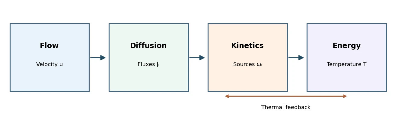
Guide 12 introduced the transport of a passive scalar. In a reactive system, the local concentration of each chemical species also depends on reaction sources or sinks. The species equations are coupled to composition, often temperature and, for compressible gases, density. Changes in temperature alter reaction rates, potentially feeding back into the temperature field.
Our case is a counter-flow methane/air diffusion flame, demonstrating practical coupling between fluid motion, mixing, reaction and energy. It is not a validated industrial reactor geometry. The workflow may transfer to other problems, but the kinetics and material properties do not automatically transfer.
Deep dive · The case in numbers: what to expect before launching the run
Before any simulation it pays to know which values are physically possible. The numbers below are computed by extra/reaction_thermo.py (section 3 box) by reading the tutorial files directly (JANAF polynomials of thermo.compressibleGas, reactions, boundary conditions in 0/, blockMeshDict) with the same formulas used by OpenFOAM 14: they are a-priori estimates, not CFD results, and serve as a yardstick for the results of the run.
| Quantity | Value | Meaning |
|---|---|---|
| heat of reaction at 298.15 K | −802.6 kJ/mol CH₄ | from the JANAF formation enthalpies in the file |
| lower heating value | 50.03 MJ/kg CH₄ | water as vapour; the factor linking Qdot to the methane consumed |
| stoichiometric mass ratio s | 3.989 kg O₂/kg CH₄ | 2·WO2/WCH4 |
| stoichiometric mixture fraction Zst | 0.0545 | air/fuel = 17.34 by mass |
| adiabatic temperature at Zst | 2305 K | complete combustion to CO₂ and H₂O, no dissociation: the upper bound of the one-step model |
| density ratio cold air / products at 2305 K | 1.184 / 0.144 = 8.2 | expansion that accelerates the flow in the reaction zone |
| convective inlet flow rates | fuel 2.634·10⁻⁵ kg/s; air 4.735·10⁻⁵ kg/s | ρ·U·A with A = 4·10⁻⁴ m² (20 × 20 mm, domain thickness included) |
| global equivalence ratio | 9.65 | the system as a whole is very rich: oxygen is the limiting reactant |
| maximum methane conversion | 10.4 % | even burning all the incoming O₂; for O₂ conversion can reach 100 % |
| maximum heat release | 136.6 W (6.83 kW per metre of depth) | upper bound for ∫Qdot dV over the whole mesh |
| global strain rate a | (0.1 + 0.1)/0.02 = 10 s⁻¹ | flow time 1/a = 0.1 s; endTime 0.5 s = 5 flow times |
| chemical time at 2000 K (stoichiometric composition) | 2.6·10⁻⁸ s | Da = 1/(a·τ) ≈ 4·10⁶: chemistry much faster than transport |
Three practical consequences. (1) A “methane conversion” of 9–10 % does not indicate slow kinetics: it is close to the maximum allowed by stoichiometry, because much more methane enters than the air can burn; oxygen conversion is the meaningful indicator. (2) With Da of the order of 10⁶ the flame is close to the infinitely fast chemistry limit (Burke–Schumann): the total heat release is controlled by the rate at which transport brings the reactants together, not by the kinetics, and changing A by a factor of 2 should shift peak temperature and integral heat release only slightly (section 7). (3) Integrated quantities of the 2D case refer to the mesh thickness, 20 mm: for values per unit depth divide by 0.02 m.
Practical tip · Mixing or reaction? The mixture fraction separates the two effects
The guide warns that a decreasing YCH4 profile does not prove conversion. The tool that separates the two effects is the mixture fraction Z, a conserved scalar (no chemical source) equal to 1 in the fuel jet and 0 in the air. It is built from the elements, which reactions neither create nor destroy; the most widely used definition is that of R. W. Bilger, S. H. Stårner, R. J. Kee, “On reduced mechanisms for methane–air combustion in nonpremixed flames”, Combustion and Flame 80, 135–149, 1990, doi:10.1016/0010-2180(90)90122-8:
beta = 2*Z_C/W_C + Z_H/(2*W_H) - Z_O/W_O        (Z_e = mass fraction of element e)
Z    = (beta - beta_air) / (beta_fuel - beta_air)
With unity Lewis number, which is the tutorial diffusion model (section 2), Z obeys the same equation as a passive tracer. At every point the methane that would be present without reaction is Z·YCH4,fuel = Z (pure methane jet): the difference Z − YCH4 is the methane consumed locally, whereas dilution lowers YCH4 and Z together. extra/paraview_profile.py (section 10) adds Z as a column to the profiles exported from ParaView; for global conversions use instead the boundary fluxes of extra/species_balance.py (section 11).
2. Conservation equations and physical meaning
The general conservative species balance for species i is:
∂(ρYᵢ)/∂t + ∇·(ρuYᵢ) = −∇·Jᵢ + ω̇ᵢ
Here Y_i is mass fraction, J_i is the diffusion flux relative to the mass-average velocity, and ωdot_i is the chemical mass source (kg·m⁻³·s⁻¹). Diffusion can depend on composition, temperature and multicomponent transport models; a single Fickian diffusivity must not be assumed for all cases. An energy equation adds enthalpy transport and the effects of chemical reactions.
Optional refresher — Advection and diffusion. Advection transports species with the moving fluid; diffusion tends to smooth composition gradients. Reactions create and consume species. A decreasing Y_CH4 profile by itself does not establish chemical conversion: dilution and mixing with air can produce the same trend.
Deep dive · The equations multicomponentFluid solves in OpenFOAM 14
The multicomponentFluid module (launched by foamRun with solver multicomponentFluid) solves species and energy in the thermophysicalPredictor() function of thermophysicalPredictor.C. Excerpt (OpenFOAM 14):
reaction->correct();

forAll(Y, i)
{
    volScalarField& Yi = Y_[i];

    if (thermo_.solveSpecie(i))
    {
        fvScalarMatrix YiEqn
        (
            fvm::ddt(rho, Yi)
          + mvConvection->fvmDiv(phi, Yi)
          + thermophysicalTransport->divj(Yi)
         ==
            reaction->R(Yi)
          + fvModels().source(rho, Yi)
        );
        ...
        YiEqn.solve("Yi");
    }
    else
    {
        Yi.correctBoundaryConditions();
    }
}

thermo_.normaliseY();

fvScalarMatrix EEqn
(
    fvm::ddt(rho, he) + mvConvection->fvmDiv(phi, he)
  + fvc::ddt(rho, K) + fvc::div(phi, K)
  + pressureWork(...)
  + thermophysicalTransport->divq(he)
 ==
    reaction->Qdot()
  + fvModels().source(rho, he)
);- It is exactly the conservative form of section 2:
fvm::ddt(rho, Yi)is ∂(ρYi)/∂t,fvmDiv(phi, Yi)is ∇·(ρuYi) withphithe mass flux on the faces [kg/s],divj(Yi)is ∇·Ji andreaction->R(Yi)is ω̇i [kg/(m³·s)], linearised. - All species use the same convection scheme,
div(phi,Yi_h)infvSchemes(the same as enthalpy): this is why thespecieFluxfunctions of section 9 must be called withschemesField=Yi_h. - The species named by
defaultSpecie N2inphysicalPropertiesis not solved: after the others,normaliseY()derives it as 1 − Σ of the others. The log therefore shows solution lines for O2, H2O, CH4 and CO2, not for N2. The balance species should be the most abundant inert one, so that closure errors are not accumulated on a minor species. - Energy is sensible enthalpy (
energy sensibleEnthalpy): chemistry enters only throughreaction->Qdot(), the source term that theQdotfunction writes as a field (section 9).Kis the kinetic energy per unit mass;pressureWorkis the pressure work (−∂p/∂t for enthalpy). - The loop is PISO:
nOuterCorrectors 1,nCorrectors 2,momentumPredictor noinfvSolution; with a single outer loop the coupling between chemistry, density and pressure within the step is explicit, which is one reason for themaxCo 0.4limit.
Deep dive · The diffusive flux Ji in the tutorial: unityLewisFourier, and how to change it
The tutorial has no constant/thermophysicalTransport. In that case laminarThermophysicalTransportModel.C selects unityLewisFourier: Fourier heat flux and species fluxes with unity Lewis number, Ji = −ρD∇Yi with ρD = κ/cp, the same coefficient for all species. The conductivity κ is that of the sutherland model with the Eucken correction (section 4). It is a strong assumption: for methane Le ≈ 0.97, so acceptable, but for hydrogen and light radicals (Le ≈ 0.3) it would be wrong; moreover a single diffusivity for all species guarantees Σ Ji = 0 without corrections.
In OpenFOAM 14 the selectable laminar models for a mixture are unityLewisFourier, FickianFourier (mixture or binary diffusivities, functions of p and T, with optional Soret thermal diffusion) and MaxwellStefanFourier (Maxwell–Stefan equations with the binary diffusivities). The syntax, from the header of FickianFourier.H, adapted to the tutorial species (the values are placeholders to be replaced with literature data):
// constant/thermophysicalTransport (only in a NEW copy)
laminar
{
    model           FickianFourier;

    mixtureDiffusionCoefficients yes;

    Dm  // [m^2/s], Function2 of p and T: a constant is accepted
    {
        CH4  2.2e-5;
        O2   2.1e-5;
        H2O  2.6e-5;
        CO2  1.6e-5;
        N2   2.0e-5;
    }
}
Two caveats. With different diffusivities the Bilger Z is no longer exactly conserved and the Burke–Schumann formulas (section 12) become an approximation. A constant diffusivity, like the placeholder, ignores the ~T1.75/p dependence: in a flame between 300 and 2300 K it must be given as a function of T. References: J. O. Hirschfelder, C. F. Curtiss, R. B. Bird, Molecular Theory of Gases and Liquids, Wiley, 1954; V. Giovangigli, Multicomponent Flow Modeling, Birkhäuser, 1999, doi:10.1007/978-1-4612-1580-6; R. J. Kee, M. E. Coltrin, P. Glarborg, Chemically Reacting Flow, Wiley, 2003, doi:10.1002/0471461296.
Orders of magnitude for the tutorial, computed by reaction_thermo.py with the Sutherland coefficients and the Eucken correction of nitrogen, the majority species:
| T [K] | μ [Pa·s] | κ [W/(m·K)] | D = κ/(ρcp) [m²/s] | cell Pe, 0.1·Δx/D | thickness δ = √(2D/a) |
|---|---|---|---|---|---|
| 293 | 1.76·10⁻⁵ | 0.0264 | 2.21·10⁻⁵ | 0.90 | 2.1 mm |
| 1000 | 4.00·10⁻⁵ | 0.0671 | 1.70·10⁻⁴ | 0.12 | 5.8 mm |
| 2000 | 5.95·10⁻⁵ | 0.109 | 5.03·10⁻⁴ | 0.04 | 10.0 mm |
The cell Péclet number is below 1 everywhere: the 0.2 mm mesh resolves molecular diffusion, and the error of the limitedLinear 1 convection scheme matters little compared with physical diffusion. The hot mixing layer, several millimetres thick, fills a large part of the 20 mm domain: this is a laminar, low-strain, very thick flame.
3. Stoichiometry, kinetics and temperature
The tutorial uses the global mechanism:
CH₄ + 2 O₂ → CO₂ + 2 H₂O
Its constant/reactions file defines an irreversibleArrhenius rate with baseline parameters A = 5.2e16, beta = 0, Ta = 14906. Ta is the activation temperature in the model’s Arrhenius representation. The units of pre-exponential factor A depend on the rate-law formulation and reaction order: do not interpret it as a first-order rate constant in s⁻¹.
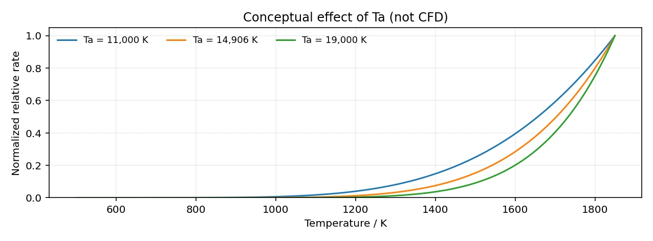
The tutorial mechanism explicitly states that it was developed for this particular flame configuration. It is not a general-purpose methane combustion mechanism, let alone a model for solution-phase kinetics.
Deep dive · The Arrhenius law in the code and the units of A
In ArrheniusReactionRateI.H the rate constant is k = A·Tβ·exp(−Ta/T):
scalar ak = A_;

if (mag(beta_) > vSmall)
{
    ak *= pow(T, beta_);
}

if (mag(Ta_) > vSmall)
{
    ak *= exp(-Ta_/T);
}

return ak;- The rate of an irreversible reaction is ω = k·Π cjej, with molar concentrations cj = ρYj/Wj in kmol/m³ (W in kg/kmol). The exponents, unless given in the string with the
CH4^0.2syntax, are the stoichiometric coefficients: here ω = k·[CH₄]·[O₂]², a third-order law. - To give ω in kmol/(m³·s), A must have units of (m³/kmol)²/s. The 5.2·10¹⁶ prefactor is therefore not comparable with a first-order k in s⁻¹, as the guide warns, nor with a literature value expressed in cm³/mol (a factor 10³ for each order above the first: 10⁶ here).
- Ta = 14906 K corresponds to an activation energy Ea = R·Ta = 123.9 kJ/mol (29.6 kcal/mol). The file can also be written with
Eaand explicit units, as the reverseBurner tutorial does (next box): OpenFOAM converts the units given in square brackets. - What a factor of 2 on A is worth. Since d(ln k)/dT = Ta/T², doubling A is equivalent to raising the temperature by ΔT = T²·ln 2/Ta: 105 K at 1500 K, 186 K at 2000 K. Experiments B and C of section 7 therefore correspond to a “kinetic” temperature change of about ±190 K in the reaction zone, a common uncertainty for a global mechanism.
Deep dive · Additional script: reaction_thermo.py, a-priori thermochemistry and kinetics from the case files
The script reads the files of a case (the tutorial or one of the prepared copies) and prints formation enthalpies, element balance, heat of reaction, heating value, Zst, adiabatic temperature with complete combustion, densities, flow rates, global equivalence ratio, limiting reactant, maximum heat release, transport properties and chemical times. Enthalpies use the janafThermo formula (dimensionless coefficients × R/W, hf evaluated at 298.15 K with the low coefficients), with R = 8314.47 J/(kmol·K). With --csv and --plot it writes the infinitely-fast-chemistry T(Z) curve. It needs only the Python standard library (matplotlib for the plot).
#!/usr/bin/env python3
"""A-priori thermochemistry of the counterFlowFlame2D case (OpenFOAM 14).

Reads constant/thermo.compressibleGas, constant/reactions, 0/CH4, 0/O2, 0/T,
0/U and system/blockMeshDict of a case (the tutorial or one of the copies made
by prepare_cases.py) and prints, with the same JANAF and Arrhenius formulas
used by OpenFOAM:

  * formation enthalpies at 298.15 K and element balance of each reaction;
  * heat of reaction and lower heating value per kg of fuel;
  * stoichiometric ratio s and stoichiometric mixture fraction Z_st;
  * adiabatic flame temperature (complete combustion, no dissociation) and
    the Burke-Schumann T(Z) curve;
  * activation energy, k(T), units of A, chemical time and Damkohler number
    against the global strain rate (U_fuel + U_air)/L;
  * density ratio between the cold inlet streams and the hot products.

Optional: --csv writes T(Z), --plot draws T(Z) (matplotlib).
Only the Python standard library is needed for the text output.
"""
import argparse, math, os, re, sys

RR = 8314.47      # J/(kmol K), universal gas constant used by OpenFOAM
TSTD = 298.15     # K, reference temperature of hf in janafThermo


def strip_comments(t):
    t = re.sub(r'/\*.*?\*/', ' ', t, flags=re.S)
    return re.sub(r'//[^\n]*', ' ', t)


def read(case, rel):
    p = os.path.join(case, rel)
    if not os.path.isfile(p):
        sys.exit('missing file: ' + p)
    return strip_comments(open(p, encoding='utf-8').read())


def block(text, name):
    """Body of the dictionary 'name { ... }' (first match, brace balanced)."""
    m = re.search(r'(?<![\w.])' + re.escape(name) + r'\s*\{', text)
    if not m:
        return None
    i, depth = m.end(), 1
    while depth:
        if text[i] == '{':
            depth += 1
        elif text[i] == '}':
            depth -= 1
        i += 1
    return text[m.end():i - 1]


def number(text, key):
    m = re.search(r'(?<![\w.])' + re.escape(key) + r'\s+([-+0-9.eE]+)\s*;', text)
    return float(m.group(1)) if m else None


def vector(text, key):
    m = re.search(r'(?<![\w.])' + re.escape(key) + r'\s*\(([^)]*)\)', text)
    return [float(v) for v in m.group(1).split()] if m else None


def species_data(case):
    t = read(case, 'constant/thermo.compressibleGas')
    names = re.search(r'species\s*\(([^)]*)\)', t).group(1).split()
    out = {}
    for n in names:
        b = block(t, n)
        out[n] = dict(W=number(b, 'molWeight'), Tlow=number(b, 'Tlow'), Thigh=number(b, 'Thigh'),
                      Tc=number(b, 'Tcommon'), hi=vector(b, 'highCpCoeffs'), lo=vector(b, 'lowCpCoeffs'),
                      As=number(b, 'As'), Ts=number(b, 'Ts'))
    return out


def ha_molar(sp, T):
    """Absolute (sensible + chemical) enthalpy, J/kmol, janafThermo::ha."""
    a = sp['hi'] if T > sp['Tc'] else sp['lo']
    return RR * (((((a[4] / 5 * T + a[3] / 4) * T + a[2] / 3) * T + a[1] / 2) * T + a[0]) * T + a[5])


def cp_molar(sp, T):
    a = sp['hi'] if T > sp['Tc'] else sp['lo']
    return RR * ((((a[4] * T + a[3]) * T + a[2]) * T + a[1]) * T + a[0])


def hf_molar(sp):
    a = sp['lo']
    T = TSTD
    return RR * (((((a[4] / 5 * T + a[3] / 4) * T + a[2] / 3) * T + a[1] / 2) * T + a[0]) * T + a[5])


def elements(formula):
    """Element counts of a simple formula such as CH4, H2O, CO2, N2."""
    out = {}
    for el, n in re.findall(r'([A-Z][a-z]?)(\d*)', formula):
        out[el] = out.get(el, 0) + (int(n) if n else 1)
    return out


def side(s):
    terms = []
    for tok in s.split('+'):
        m = re.match(r'\s*([0-9.]*)\s*([A-Za-z][A-Za-z0-9]*)(?:\^([0-9.]+))?\s*$', tok)
        if not m:
            sys.exit('cannot parse reaction term: ' + tok)
        terms.append((float(m.group(1)) if m.group(1) else 1.0, m.group(2),
                      float(m.group(3)) if m.group(3) else None))
    return terms


def reactions(case):
    t = read(case, 'constant/reactions')
    body = block(t, 'reactions')
    out = []
    for m in re.finditer(r'(\w+)\s*\{', body):
        b = block(body, m.group(1))
        if b is None or 'reaction' not in b:
            continue
        eq = re.search(r'reaction\s+"([^"]+)"', b).group(1)
        typ = re.search(r'type\s+(\w+)\s*;', b).group(1)
        lhs, rhs = eq.split('=')
        out.append(dict(name=m.group(1), type=typ, eq=eq, lhs=side(lhs), rhs=side(rhs),
                        A=number(b, 'A'), beta=number(b, 'beta'), Ta=number(b, 'Ta')))
    return out


def patch_value(case, field, patch):
    t = read(case, '0/' + field)
    b = block(block(t, 'boundaryField'), patch)
    m = re.search(r'(?:value|inletValue)\s+uniform\s+(\([^)]*\)|[-+0-9.eE]+)', b)
    v = m.group(1)
    return [float(x) for x in v.strip('()').split()] if v.startswith('(') else float(v)


def internal_value(case, field):
    t = read(case, '0/' + field)
    m = re.search(r'internalField\s+uniform\s+([-+0-9.eE]+)', t)
    return float(m.group(1))


def domain_length(case):
    t = read(case, 'system/blockMeshDict')
    conv = number(t, 'convertToMeters') or 1.0
    xs = [float(v.split()[0]) for v in re.findall(r'\(\s*([-+0-9.eE]+\s+[-+0-9.eE]+\s+[-+0-9.eE]+)\s*\)',
                                                   block_list(t, 'vertices'))]
    return (max(xs) - min(xs)) * conv


def vertices(case):
    t = read(case, 'system/blockMeshDict')
    conv = number(t, 'convertToMeters') or 1.0
    return t, [[conv * float(c) for c in v.split()] for v in
               re.findall(r'\(\s*([-+0-9.eE]+\s+[-+0-9.eE]+\s+[-+0-9.eE]+)\s*\)', block_list(t, 'vertices'))]


def patch_area(case, patch):
    """Area of a blockMesh patch made of planar quadrilateral faces (half the cross product of the diagonals)."""
    t, V = vertices(case)
    b = block(block_list(t, 'boundary'), patch)
    if b is None:
        return None
    area = 0.0
    for f in re.findall(r'\(\s*(\d+)\s+(\d+)\s+(\d+)\s+(\d+)\s*\)', b):
        p0, p1, p2, p3 = (V[int(i)] for i in f)
        d1 = [p2[i] - p0[i] for i in range(3)]
        d2 = [p3[i] - p1[i] for i in range(3)]
        cr = [d1[1] * d2[2] - d1[2] * d2[1], d1[2] * d2[0] - d1[0] * d2[2], d1[0] * d2[1] - d1[1] * d2[0]]
        area += 0.5 * math.sqrt(sum(c * c for c in cr))
    return area


def block_list(text, name):
    m = re.search(name + r'\s*\(', text)
    i, depth = m.end(), 1
    while depth:
        depth += {'(': 1, ')': -1}.get(text[i], 0)
        i += 1
    return text[m.end():i - 1]


def mix_h(Y, sp, T):
    """Mass-specific absolute enthalpy of a mixture, J/kg."""
    return sum(Y[n] * ha_molar(sp[n], T) / sp[n]['W'] for n in Y if Y[n])


def mix_W(Y, sp):
    return 1.0 / sum(Y[n] / sp[n]['W'] for n in Y if Y[n])


def solve_T(Y, sp, h, T0=1500.0):
    T = T0
    for _ in range(100):
        f = mix_h(Y, sp, T) - h
        cp = sum(Y[n] * cp_molar(sp[n], T) / sp[n]['W'] for n in Y if Y[n])
        dT = -f / cp
        T += dT
        if abs(dT) < 1e-6:
            return T
    raise RuntimeError('temperature iteration did not converge')


def main():
    ap = argparse.ArgumentParser(description=__doc__.split('\n')[0])
    ap.add_argument('case', help='case directory (tutorial copy)')
    ap.add_argument('--fuel', default='CH4')
    ap.add_argument('--oxidiser', default='O2')
    ap.add_argument('--inert', default='N2')
    ap.add_argument('--fuel-patch', default='fuel')
    ap.add_argument('--air-patch', default='air')
    ap.add_argument('--temperatures', default='1000,1500,1800,2000,2200',
                    help='comma-separated temperatures for k(T) and the chemical time')
    ap.add_argument('--csv', help='write the Burke-Schumann T(Z) curve to this CSV')
    ap.add_argument('--plot', help='write a PNG of T(Z) (needs matplotlib)')
    ap.add_argument('--lang', choices=('it', 'en'), default='en', help='language of the plot labels')
    a = ap.parse_args()

    sp = species_data(a.case)
    print('Species (molWeight kg/kmol, hf(298.15 K) kJ/mol):')
    for n, d in sp.items():
        print(f'  {n:4s} W = {d["W"]:8.4f}   hf = {hf_molar(d) / 1e6:9.2f}')

    F, O, N = a.fuel, a.oxidiser, a.inert
    for r in reactions(a.case):
        print(f'\nReaction {r["name"]} ({r["type"]}): {r["eq"]}')
        bal = {}
        for sgn, terms in ((-1, r['lhs']), (1, r['rhs'])):
            for nu, s, _ in terms:
                for el, k in elements(s).items():
                    bal[el] = bal.get(el, 0) + sgn * nu * k
        print('  element balance (products - reactants):', ', '.join(f'{e} {v:+g}' for e, v in sorted(bal.items())),
              '-> OK' if all(abs(v) < 1e-12 for v in bal.values()) else '-> NOT BALANCED')
        dH = sum(nu * hf_molar(sp[s]) for nu, s, _ in r['rhs']) - sum(nu * hf_molar(sp[s]) for nu, s, _ in r['lhs'])
        nuF = next(nu for nu, s, _ in r['lhs'] if s == F)
        nuO = next(nu for nu, s, _ in r['lhs'] if s == O)
        print(f'  heat of reaction at 298.15 K: {dH / 1e6 / nuF:.1f} kJ per mol {F}')
        LHV = -dH / nuF / sp[F]['W']
        print(f'  lower heating value (H2O as vapour): {LHV / 1e6:.2f} MJ per kg {F}')
        order = sum((e if e is not None else nu) for nu, s, e in r['lhs'])
        Ea = RR * r['Ta']
        print(f'  Arrhenius: k = A T^beta exp(-Ta/T), A = {r["A"]:.4g}, beta = {r["beta"]:g}, Ta = {r["Ta"]:g} K')
        print(f'  activation energy Ea = R Ta = {Ea / 1e6:.1f} kJ/mol = {Ea / 4.184e6:.1f} kcal/mol')
        print('  rate exponents (default = stoichiometric coefficients): ' +
              ', '.join(f'{s}^{e if e is not None else nu:g}' for nu, s, e in r['lhs']) + f'  -> overall order {order:g}')
        print(f'  units of A (concentrations in kmol/m3): (m3/kmol)^{order - 1:g} / s'
              + ('' if not r['beta'] else ' / K^beta'))
        print(f'  a factor 2 on A is equivalent to a temperature change dT = T^2 ln2 / Ta: '
              + ', '.join(f'{T:.0f} K -> {T * T * math.log(2) / r["Ta"]:.0f} K' for T in (1500, 2000)))

        s_mass = nuO * sp[O]['W'] / (nuF * sp[F]['W'])
        YF1 = patch_value(a.case, F, a.fuel_patch)
        YO2 = patch_value(a.case, O, a.air_patch)
        YN_air = patch_value(a.case, N, a.air_patch)
        YN_fuel = patch_value(a.case, N, a.fuel_patch)
        T1 = patch_value(a.case, 'T', a.fuel_patch)
        T2 = patch_value(a.case, 'T', a.air_patch)
        print(f'\nInlet streams: fuel Y_{F} = {YF1:g}, Y_{N} = {YN_fuel:g}, T = {T1:g} K;'
              f' air Y_{O} = {YO2:g}, Y_{N} = {YN_air:g}, T = {T2:g} K')
        Zst = YO2 / (s_mass * YF1 + YO2)
        print(f'  stoichiometric mass ratio s = nu_O W_O / (nu_F W_F) = {s_mass:.4f} kg {O} per kg {F}')
        print(f'  stoichiometric mixture fraction Z_st = Y_O,air / (s Y_F,fuel + Y_O,air) = {Zst:.4f}')
        print(f'  equivalent fuel/air mass ratio at Z_st = {Zst / (1 - Zst):.4f}  (air/fuel = {(1 - Zst) / Zst:.2f})')

        prod = [s for _, s, _ in r['rhs']]

        def state(Z, burnt):
            Y = {n: 0.0 for n in sp}
            Y[F] = YF1 * Z
            Y[O] = YO2 * (1 - Z)
            Y[N] = YN_fuel * Z + YN_air * (1 - Z)
            h = Z * mix_h({F: YF1, N: YN_fuel}, sp, T1) + (1 - Z) * mix_h({O: YO2, N: YN_air}, sp, T2)
            if burnt:
                ext = min(Y[F] / (nuF * sp[F]['W']), Y[O] / (nuO * sp[O]['W']))  # kmol of 'reaction' per kg
                for nu, s, _ in r['lhs']:
                    Y[s] -= nu * ext * sp[s]['W']
                for nu, s, _ in r['rhs']:
                    Y[s] += nu * ext * sp[s]['W']
                Y = {k: max(v, 0.0) for k, v in Y.items()}
            return Y, h

        Yb, h = state(Zst, True)
        Tad = solve_T(Yb, sp, h, 2000.0)
        print(f'\nAdiabatic flame temperature at Z_st (complete combustion, no dissociation, p const): {Tad:.0f} K')
        print('  burnt composition at Z_st: ' + ', '.join(f'{n} {v:.4f}' for n, v in Yb.items() if v > 1e-12))
        Wb = mix_W(Yb, sp)
        Ya, _ = state(0.0, False)
        Wa = mix_W(Ya, sp)
        p = internal_value(a.case, 'p')
        rho_air = p * Wa / (RR * T2)
        rho_b = p * Wb / (RR * Tad)
        print(f'  density: cold air {rho_air:.3f} kg/m3, products at Tad {rho_b:.4f} kg/m3, ratio {rho_air / rho_b:.2f}')
        Yf, _ = state(1.0, False)
        print(f'  density of the cold fuel stream: {p * mix_W(Yf, sp) / (RR * T1):.3f} kg/m3')

        UF = patch_value(a.case, 'U', a.fuel_patch)[0]
        UA = patch_value(a.case, 'U', a.air_patch)[0]
        AF, AA = patch_area(a.case, a.fuel_patch), patch_area(a.case, a.air_patch)
        rhoF = p * mix_W(Yf, sp) / (RR * T1)
        mF, mA = rhoF * abs(UF) * AF, rho_air * abs(UA) * AA
        print(f'\nInlet mass flows (convective, rho U A; diffusion through the inlet faces is not included):')
        print(f'  fuel: A = {AF:.4g} m2, {mF:.4e} kg/s ({mF * YF1:.4e} kg/s {F})')
        print(f'  air : A = {AA:.4g} m2, {mA:.4e} kg/s ({mA * YO2:.4e} kg/s {O})')
        Zg = mF / (mF + mA)
        phi_g = (mF * YF1 / (mA * YO2)) * s_mass
        print(f'  global mixture fraction {Zg:.4f} (Z_st = {Zst:.4f}), global equivalence ratio {phi_g:.2f}')
        if phi_g > 1:
            mFmax = mA * YO2 / s_mass
            print(f'  {O} is the limiting reactant: at most {mFmax:.4e} kg/s of {F} can burn,'
                  f' i.e. a maximum {F} conversion of {100 * mFmax / (mF * YF1):.1f} %; {O} conversion can reach 100 %')
        else:
            mFmax = mF * YF1
            print(f'  {F} is the limiting reactant: {O} conversion at most {100 * phi_g:.1f} %')
        print(f'  upper bound of the heat release (complete combustion of the limiting reactant): {mFmax * LHV:.1f} W'
              f' for the simulated depth (whole mesh)')
        Ld = domain_length(a.case)
        strain = (abs(UF) + abs(UA)) / Ld
        print(f'\nGlobal strain rate a = (|U_fuel| + |U_air|) / L = ({abs(UF):g} + {abs(UA):g}) / {Ld:g} = {strain:.3g} 1/s'
              f'  (flow time 1/a = {1 / strain:.3g} s)')

        n_x = int(re.search(r'hex\s*\([^)]*\)\s*\(\s*(\d+)', read(a.case, 'system/blockMeshDict')).group(1))
        dx = Ld / n_x
        print(f'Transport with unityLewisFourier (D = kappa/(rho cp), Le = 1), estimated with the {N} Sutherland/Eucken data'
              f' (the majority species); cell size dx = {dx:.3g} m:')
        print('     T [K]      mu [Pa s]   kappa [W/m/K]   D = alpha [m2/s]   cell Pe = 0.1 dx/D   delta = sqrt(2D/a) [mm]')
        dN = sp[N]
        for T in (T2, 1000.0, 1500.0, 2000.0, Tad):
            mu = dN['As'] * math.sqrt(T) / (1 + dN['Ts'] / T)
            cp = cp_molar(dN, T) / dN['W']
            cv = cp - RR / dN['W']
            kap = mu * cv * (1.32 + 1.77 * (RR / dN['W']) / cv)
            rho = p * dN['W'] / (RR * T)
            al = kap / (rho * cp)
            print(f'  {T:8.0f}   {mu:10.4e}   {kap:12.4e}   {al:14.4e}   {0.1 * dx / al:16.3f}   {1e3 * math.sqrt(2 * al / strain):18.2f}')
        print('  (delta is the thickness of the strained mixing layer: compare it with dx to judge the resolution)')

        Yu, _ = state(Zst, False)
        Wu = mix_W(Yu, sp)
        print(f'Chemical time of {F} at the stoichiometric unburnt composition, p = {p:g} Pa:')
        print('     T [K]        k [(m3/kmol)^' + f'{order - 1:g}/s]   [{F}] [kmol/m3]   tau_chem [s]    Da = 1/(a tau)')
        for T in [float(v) for v in a.temperatures.split(',')]:
            k = r['A'] * T ** r['beta'] * math.exp(-r['Ta'] / T)
            rho = p * Wu / (RR * T)
            conc = {s: rho * Yu[s] / sp[s]['W'] for s in sp}
            w = k * math.prod(conc[s] ** (e if e is not None else nu) for nu, s, e in r['lhs'])   # kmol/m3/s of reaction
            tau = conc[F] / (nuF * w)
            print(f'  {T:8.0f}   {k:14.4e}   {conc[F]:14.4e}   {tau:12.4e}   {1 / (strain * tau):12.4e}')
        print('  (order-of-magnitude indicator only: in the flame the composition is diluted by products'
              ' and diffusion, so the effective time is longer)')

        if a.csv or a.plot:
            rows = []
            for i in range(201):
                Z = i / 200
                Yb_, h_ = state(Z, True)
                Yu_, _ = state(Z, False)
                rows.append((Z, solve_T(Yb_, sp, h_, 1500.0), solve_T(Yu_, sp, h_, 300.0), Yb_[F], Yb_[O], *[Yb_[s] for s in prod]))
            if a.csv:
                with open(a.csv, 'w', encoding='utf-8') as f:
                    f.write('Z,T_burnt_K,T_mixing_K,Y_' + F + ',Y_' + O + ',' + ','.join('Y_' + s for s in prod) + '\n')
                    for row in rows:
                        f.write(','.join(f'{v:.6g}' for v in row) + '\n')
                print('\nwritten', a.csv)
            if a.plot:
                import matplotlib
                matplotlib.use('Agg')
                import matplotlib.pyplot as plt
                it = a.lang == 'it'
                fig, ax = plt.subplots(figsize=(8, 4.6), dpi=150)
                ax.plot([r_[0] for r_ in rows], [r_[1] for r_ in rows], color='#c0392b', lw=2,
                        label='combustione completa (Burke–Schumann)' if it else 'complete combustion (Burke–Schumann)')
                ax.plot([r_[0] for r_ in rows], [r_[2] for r_ in rows], color='#2c6fbb', lw=1.5, ls='--',
                        label='miscelamento senza reazione' if it else 'mixing without reaction')
                ax.axvline(Zst, color='#555', lw=1, ls=':')
                ax.annotate(f'Z_st = {Zst:.4f}\nT_ad = {Tad:.0f} K', (Zst, Tad), xytext=(Zst + 0.08, Tad - 250),
                            arrowprops=dict(arrowstyle='->', color='#555'), fontsize=9)
                ax.set_xlabel('frazione di miscela Z [-]' if it else 'mixture fraction Z [-]')
                ax.set_ylabel('T [K]')
                ax.set_xlim(0, 1)
                ax.set_ylim(0, 2600)
                ax.grid(alpha=0.3)
                ax.legend(fontsize=9, loc='upper right')
                ax.set_title(('Temperatura di equilibrio a chimica infinitamente veloce, ' if it else 'Infinitely fast chemistry temperature, ')
                             + os.path.basename(os.path.abspath(a.case)), fontsize=10)
                fig.tight_layout()
                fig.savefig(a.plot)
                print('written', a.plot)


if __name__ == '__main__':
    main()
Run on the three copies prepared by prepare_cases.py (for B and C only the lines that change):
$ python3 reaction_thermo.py A_reference --csv tz.csv --plot tz_en.png
Species (molWeight kg/kmol, hf(298.15 K) kJ/mol):
  O2   W =  31.9988   hf =     -0.00
  H2O  W =  18.0153   hf =   -241.85
  CH4  W =  16.0428   hf =    -74.60
  CO2  W =  44.0100   hf =   -393.55
  N2   W =  28.0134   hf =      0.00

Reaction methaneReaction (irreversibleArrhenius): CH4 + 2O2 = CO2 + 2H2O
  element balance (products - reactants): C +0, H +0, O +0 -> OK
  heat of reaction at 298.15 K: -802.6 kJ per mol CH4
  lower heating value (H2O as vapour): 50.03 MJ per kg CH4
  Arrhenius: k = A T^beta exp(-Ta/T), A = 5.2e+16, beta = 0, Ta = 14906 K
  activation energy Ea = R Ta = 123.9 kJ/mol = 29.6 kcal/mol
  rate exponents (default = stoichiometric coefficients): CH4^1, O2^2  -> overall order 3
  units of A (concentrations in kmol/m3): (m3/kmol)^2 / s
  a factor 2 on A is equivalent to a temperature change dT = T^2 ln2 / Ta: 1500 K -> 105 K, 2000 K -> 186 K

Inlet streams: fuel Y_CH4 = 1, Y_N2 = 0, T = 293 K; air Y_O2 = 0.23, Y_N2 = 0.77, T = 293 K
  stoichiometric mass ratio s = nu_O W_O / (nu_F W_F) = 3.9892 kg O2 per kg CH4
  stoichiometric mixture fraction Z_st = Y_O,air / (s Y_F,fuel + Y_O,air) = 0.0545
  equivalent fuel/air mass ratio at Z_st = 0.0577  (air/fuel = 17.34)

Adiabatic flame temperature at Z_st (complete combustion, no dissociation, p const): 2305 K
  burnt composition at Z_st: H2O 0.1224, CO2 0.1495, N2 0.7280
  density: cold air 1.184 kg/m3, products at Tad 0.1442 kg/m3, ratio 8.21
  density of the cold fuel stream: 0.659 kg/m3

Inlet mass flows (convective, rho U A; diffusion through the inlet faces is not included):
  fuel: A = 0.0004 m2, 2.6341e-05 kg/s (2.6341e-05 kg/s CH4)
  air : A = 0.0004 m2, 4.7353e-05 kg/s (1.0891e-05 kg/s O2)
  global mixture fraction 0.3574 (Z_st = 0.0545), global equivalence ratio 9.65
  O2 is the limiting reactant: at most 2.7302e-06 kg/s of CH4 can burn, i.e. a maximum CH4 conversion of 10.4 %; O2 conversion can reach 100 %
  upper bound of the heat release (complete combustion of the limiting reactant): 136.6 W for the simulated depth (whole mesh)

Global strain rate a = (|U_fuel| + |U_air|) / L = (0.1 + 0.1) / 0.02 = 10 1/s  (flow time 1/a = 0.1 s)
Transport with unityLewisFourier (D = kappa/(rho cp), Le = 1), estimated with the N2 Sutherland/Eucken data (the majority species); cell size dx = 0.0002 m:
     T [K]      mu [Pa s]   kappa [W/m/K]   D = alpha [m2/s]   cell Pe = 0.1 dx/D   delta = sqrt(2D/a) [mm]
       293   1.7566e-05     2.6399e-02       2.2132e-05              0.904                 2.10
      1000   4.0021e-05     6.7128e-02       1.7036e-04              0.117                 5.84
      1500   5.0648e-05     8.9829e-02       3.2188e-04              0.062                 8.02
      2000   5.9473e-05     1.0880e-01       5.0271e-04              0.040                10.03
      2305   6.4274e-05     1.1893e-01       6.2549e-04              0.032                11.18
  (delta is the thickness of the strained mixing layer: compare it with dx to judge the resolution)
Chemical time of CH4 at the stoichiometric unburnt composition, p = 100000 Pa:
     T [K]        k [(m3/kmol)^2/s]   [CH4] [kmol/m3]   tau_chem [s]    Da = 1/(a tau)
      1000       1.7475e+10       1.1295e-03     1.1214e-05     8.9176e+03
      1500       2.5135e+12       7.5300e-04     1.7542e-07     5.7007e+05
      1800       1.3169e+13       6.2750e-04     4.8211e-08     2.0742e+06
      2000       3.0144e+13       5.6475e-04     2.6003e-08     3.8458e+06
      2200       5.9355e+13       5.1341e-04     1.5979e-08     6.2582e+06
  (order-of-magnitude indicator only: in the flame the composition is diluted by products and diffusion, so the effective time is longer)

written tz.csv
written tz_en.png
$ python3 reaction_thermo.py B_half_A   # excerpt: chemical time table and Arrhenius line
     T [K]        k [(m3/kmol)^2/s]   [CH4] [kmol/m3]   tau_chem [s]    Da = 1/(a tau)
      1000       8.7374e+09       1.1295e-03     2.2428e-05     4.4588e+03
      1500       1.2567e+12       7.5300e-04     3.5083e-07     2.8503e+05
      1800       6.5846e+12       6.2750e-04     9.6422e-08     1.0371e+06
      2000       1.5072e+13       5.6475e-04     5.2005e-08     1.9229e+06
      2200       2.9678e+13       5.1341e-04     3.1958e-08     3.1291e+06
  (order-of-magnitude indicator only: in the flame the composition is diluted by products and diffusion, so the effective time is longer)
  Arrhenius: k = A T^beta exp(-Ta/T), A = 2.6e+16, beta = 0, Ta = 14906 K
$ python3 reaction_thermo.py C_double_A   # excerpt: chemical time table and Arrhenius line
     T [K]        k [(m3/kmol)^2/s]   [CH4] [kmol/m3]   tau_chem [s]    Da = 1/(a tau)
      1000       3.4949e+10       1.1295e-03     5.6069e-06     1.7835e+04
      1500       5.0269e+12       7.5300e-04     8.7709e-08     1.1401e+06
      1800       2.6339e+13       6.2750e-04     2.4106e-08     4.1484e+06
      2000       6.0289e+13       5.6475e-04     1.3001e-08     7.6915e+06
      2200       1.1871e+14       5.1341e-04     7.9895e-09     1.2516e+07
  (order-of-magnitude indicator only: in the flame the composition is diluted by products and diffusion, so the effective time is longer)
  Arrhenius: k = A T^beta exp(-Ta/T), A = 1.04e+17, beta = 0, Ta = 14906 K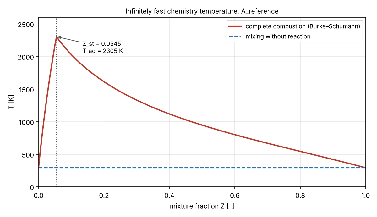
Infinitely fast chemistry T(Z) curve (Burke–Schumann) written by reaction_thermo.py with the tutorial JANAF data; the dashed line is pure mixing at 293 K. Theoretical estimate, not a CFD result.
Reading the results: the chemical time τ drops by three orders of magnitude between 1000 and 2000 K and stays at 10⁻⁸–10⁻⁷ s in the hot zone, much shorter than the initial time step (10⁻⁶ s) and the later ones set by maxCo: this is why the chemistry is integrated by an implicit ODE solver with its own sub-steps (section 14). The values for B and C are exactly twice and half the τ of A, as expected from linearity in A.
Deep dive · Global mechanisms: why the tutorial one is not transferable
The constant/reactions file gives as its source the PhD thesis of M. N. Bui-Pham (University of California, San Diego, 1992) and warns that the mechanism was developed for this configuration. OpenFOAM 14 contains a second global methane mechanism, in the multiRegion/CHT/reverseBurner tutorial: it is set 3 of table 2 of C. K. Westbrook, F. L. Dryer, “Simplified reaction mechanisms for the oxidation of hydrocarbon fuels in flames”, Combustion Science and Technology 27, 31–43, 1981, doi:10.1080/00102208108946970:
methaneReaction
{
    type    irreversibleArrhenius;
    reaction "CH4^0.2 + 2O2^1.3 = CO2 + 2H2O";
    A       6.7e12 [(mol/cm^3)^-0.5/s];
    beta    0;
    Ea      48.4 [kcal/mol];
}
Converted to internal units, A = 6.7·10¹² × 1000−0.5 = 2.12·10¹¹ (m³/kmol)0.5/s and Ta = 24 356 K. At the stoichiometric composition, at 1 bar, the two laws give very different rates (kmol/(m³·s), computed with the formulas of the previous box):
| T [K] | counterFlowFlame2D (Bui-Pham) | reverseBurner (Westbrook–Dryer) | ratio |
|---|---|---|---|
| 1000 | 1.0·10² | 5.2·10⁻⁴ | 1.9·10⁵ |
| 1500 | 4.3·10³ | 0.96 | 4.5·10³ |
| 2000 | 2.2·10⁴ | 36 | 600 |
| 2200 | 3.2·10⁴ | 94 | 340 |
A difference of two to five orders of magnitude between two “methane” laws shows that global parameters are tuning parameters: Westbrook and Dryer chose theirs to reproduce premixed flame speeds and flammability limits, the tutorial mechanism was built for this diffusion flame. In a high-Damköhler diffusion flame the difference matters little for the total heat release, but it changes ignition, reaction-zone thickness and behaviour near extinction. A global mechanism produces no CO and H₂ and has no dissociation, so it overestimates the peak temperature (2305 K against about 2220 K from a chemical equilibrium calculation with dissociation). For other reduced mechanisms: W. P. Jones, R. P. Lindstedt, “Global reaction schemes for hydrocarbon combustion”, Combustion and Flame 73, 233–249, 1988, doi:10.1016/0010-2180(88)90021-1; for the detailed mechanism, GRI-Mech 3.0 (53 species, 325 reactions), used by the _GRI variants of the tutorial (section 4).
4. The official OpenFOAM Foundation 14 case
Source case: tutorials/multicomponentFluid/counterFlowFlame2D. The relevant files have been checked in the Foundation 14 repository.
| File | Purpose | Caution |
|---|---|---|
system/controlDict | solver multicomponentFluid, step size and output | run with foamRun |
0/CH4, 0/O2, 0/N2 | initial and boundary composition | mass fractions |
0/T, 0/U, 0/p | temperature, velocity and pressure | T in K, p in Pa |
constant/physicalProperties | multicomponent thermodynamics | hePsiThermo, perfectGas |
constant/thermo.compressibleGas | thermophysical species data | not valid for liquids |
constant/chemistryProperties | chemistry integration | ode/solver seulex |
constant/reactionProperties | reaction model | reactionModel laminar |
constant/reactions | stoichiometry and Arrhenius law | edit copies only |
system/functions | diagnostic functions | includes Qdot |
Version note. These files describe OpenFOAM Foundation 14. Tutorials using reactingFoam, thermophysicalProperties or chemistryReader in other releases/distributions are not necessarily interchangeable.
Deep dive · All the counterFlowFlame2D tutorial files, as they are in version 14
File contents (without headers), to be compared with the copy on the server before any change. The complete case is in the version 14 repository. The tutorial has no Allrun: the sequence is blockMesh and foamRun, which is what run_case.sh runs (section 8).
Allclean
#!/bin/sh
cd ${0%/*} || exit 1    # Run from this directory

# Source tutorial clean functions
. $WM_PROJECT_DIR/bin/tools/CleanFunctions

cleanCase && rm -rf 0/Qdot

#------------------------------------------------------------------------------
0/CH4
dimensions      [];

internalField   uniform 0;

boundaryField
{
    #includeEtc "caseDicts/setConstraintTypes"

    fuel
    {
        type            fixedValue;
        value           uniform 1;
    }
    air
    {
        type            fixedValue;
        value           uniform 0;
    }
    outlet
    {
        type            inletOutlet;
        inletValue      uniform 0;
    }
}
0/O2
dimensions      [];

internalField   uniform 0;

boundaryField
{
    #includeEtc "caseDicts/setConstraintTypes"

    fuel
    {
        type            fixedValue;
        value           uniform 0;
    }
    air
    {
        type            fixedValue;
        value           uniform 0.23;
    }
    outlet
    {
        type            inletOutlet;
        inletValue      uniform 0;
    }
}
0/N2
dimensions      [];

internalField   uniform 1;

boundaryField
{
    #includeEtc "caseDicts/setConstraintTypes"

    fuel
    {
        type            fixedValue;
        value           uniform 0;
    }
    air
    {
        type            fixedValue;
        value           uniform 0.77;
    }
    outlet
    {
        type            inletOutlet;
        inletValue      uniform 1;
    }
}
0/Ydefault
dimensions      [];

internalField   uniform 0;

boundaryField
{
    #includeEtc "caseDicts/setConstraintTypes"

    fuel
    {
        type            fixedValue;
        value           uniform 0;
    }
    air
    {
        type            fixedValue;
        value           uniform 0;
    }
    outlet
    {
        type            inletOutlet;
        inletValue      uniform 0;
    }
}
0/T
dimensions      [temperature];

internalField   uniform 2000;

boundaryField
{
    #includeEtc "caseDicts/setConstraintTypes"

    fuel
    {
        type            fixedValue;
        value           uniform 293;
    }
    air
    {
        type            fixedValue;
        value           uniform 293;
    }
    outlet
    {
        type            inletOutlet;
        inletValue      uniform 293;
    }
}
0/U
dimensions      [velocity];

internalField   uniform (0 0 0);

boundaryField
{
    #includeEtc "caseDicts/setConstraintTypes"

    fuel
    {
        type            fixedValue;
        value           uniform (0.1 0 0);
    }
    air
    {
        type            fixedValue;
        value           uniform (-0.1 0 0);
    }
    outlet
    {
        type            pressureInletOutletVelocity;
    }
}
0/p
dimensions      [pressure];

internalField   uniform 1e5;

boundaryField
{
    #includeEtc "caseDicts/setConstraintTypes"

    fuel
    {
        type            zeroGradient;
    }
    air
    {
        type            zeroGradient;
    }
    outlet
    {
        type            totalPressure;
        p0              $internalField;
    }
}constant/physicalProperties, constant/momentumTransport, constant/reactionProperties
thermoType
{
    type            hePsiThermo;
    mixture         coefficientWilkeMulticomponentMixture;
    transport       sutherland;
    thermo          janaf;
    energy          sensibleEnthalpy;
    equationOfState perfectGas;
    specie          specie;
}

defaultSpecie N2;

#include "thermo.compressibleGas"

simulationType  laminar;

reactionModel  laminar;
constant/chemistryProperties
initialChemicalTimeStep 1e-07;

ode
{
    solver          seulex;
    absTol          1e-8;
    relTol          1e-1;
}

#include "reactions"
constant/reactions (with the original header comment)
Reference:
    Bui-Pham, M. N. (1992).
    Studies in structures of lam inar hydrocarbon flames.
    PhD Thesis, University of California, San Diego

Notes:
    This mechanism was developed for simulating this exact counter-flow flame
    configuration. It should not be considered general-purpose.


reactions
{
    methaneReaction
    {
        type     irreversibleArrhenius;
        reaction "CH4 + 2O2 = CO2 + 2H2O";
        A        5.2e16;
        beta     0;
        Ta       14906;
    }
}
constant/thermo.compressibleGas
species
(
    O2
    H2O
    CH4
    CO2
    N2
);

O2
{
    specie
    {
        molWeight       31.9988;
    }
    thermodynamics
    {
        Tlow            200;
        Thigh           5000;
        Tcommon         1000;
        highCpCoeffs    ( 3.69758 0.00061352 -1.25884e-07 1.77528e-11 -1.13644e-15 -1233.93 3.18917 );
        lowCpCoeffs     ( 3.21294 0.00112749 -5.75615e-07 1.31388e-09 -8.76855e-13 -1005.25 6.03474 );
    }
    transport
    {
        As              1.753e-6;
        Ts              139;
    }
}

H2O
{
    specie
    {
        molWeight       18.0153;
    }
    thermodynamics
    {
        Tlow            200;
        Thigh           5000;
        Tcommon         1000;
        highCpCoeffs    ( 2.67215 0.00305629 -8.73026e-07 1.201e-10 -6.39162e-15 -29899.2 6.86282 );
        lowCpCoeffs     ( 3.38684 0.00347498 -6.3547e-06 6.96858e-09 -2.50659e-12 -30208.1 2.59023 );
    }
    transport
    {
        As              2.978e-7;
        Ts              1064;
    }
}

CH4
{
    specie
    {
        molWeight       16.0428;
    }
    thermodynamics
    {
        Tlow            200;
        Thigh           6000;
        Tcommon         1000;
        highCpCoeffs    ( 1.63543 0.0100844 -3.36924e-06 5.34973e-10 -3.15528e-14 -10005.6 9.9937 );
        lowCpCoeffs     ( 5.14988 -0.013671 4.91801e-05 -4.84744e-08 1.66694e-11 -10246.6 -4.64132 );
    }
    transport
    {
        As              1.0194e-06;
        Ts              171.06;
    }
}

CO2
{
    specie
    {
        molWeight       44.01;
    }
    thermodynamics
    {
        Tlow            200;
        Thigh           5000;
        Tcommon         1000;
        highCpCoeffs    ( 4.45362 0.00314017 -1.27841e-06 2.394e-10 -1.66903e-14 -48967 -0.955396 );
        lowCpCoeffs     ( 2.27572 0.00992207 -1.04091e-05 6.86669e-09 -2.11728e-12 -48373.1 10.1885 );
    }
    transport
    {
        As              1.503e-6;
        Ts              222;
    }
}

N2
{
    specie
    {
        molWeight       28.0134;
    }
    thermodynamics
    {
        Tlow            200;
        Thigh           5000;
        Tcommon         1000;
        highCpCoeffs    ( 2.92664 0.00148798 -5.68476e-07 1.0097e-10 -6.75335e-15 -922.798 5.98053 );
        lowCpCoeffs     ( 3.29868 0.00140824 -3.96322e-06 5.64152e-09 -2.44486e-12 -1020.9 3.95037 );
    }
    transport
    {
        As              1.401e-6;
        Ts              107;
    }
}system/controlDict, system/functions
solver          multicomponentFluid;

startFrom       startTime;

startTime       0;

stopAt          endTime;

endTime         0.5;

deltaT          1e-6;

writeControl    adjustableRunTime;

writeInterval   0.05;

purgeWrite      0;

writeFormat     ascii;

writePrecision  6;

writeCompression off;

timeFormat      general;

timePrecision   6;

runTimeModifiable true;

adjustTimeStep  yes;

maxCo           0.4;

#includeFunc Qdot
system/blockMeshDict
vertices
(
    (0.0  -0.01 -0.01)
    (0.02 -0.01 -0.01)
    (0.02  0.01 -0.01)
    (0.0   0.01 -0.01)
    (0.0  -0.01  0.01)
    (0.02 -0.01  0.01)
    (0.02  0.01  0.01)
    (0.0   0.01  0.01)
);

blocks
(
    hex (0 1 2 3 4 5 6 7) (100 40 1) simpleGrading (1 1 1)
);

boundary
(
    fuel
    {
        type patch;
        faces
        (
            (0 4 7 3)
        );
    }
    air
    {
        type patch;
        faces
        (
            (1 2 6 5)
        );
    }
    outlet
    {
        type patch;
        faces
        (
            (0 1 5 4)
            (7 6 2 3)
        );
    }
    frontAndBack
    {
        type empty;
        faces
        (
            (4 5 6 7)
            (0 3 2 1)
        );
    }
);
system/fvSchemes
ddtSchemes
{
    default         Euler;
}

gradSchemes
{
    default         Gauss linear;
}

divSchemes
{
    default         none;

    div(phi,U)      Gauss limitedLinearV 1;
    div(phi,Yi_h)   Gauss limitedLinear 1;
    div(phi,K)      Gauss limitedLinear 1;
    div(phid,p)     Gauss limitedLinear 1;
    div(phi,epsilon) Gauss limitedLinear 1;
    div(phi,k) Gauss limitedLinear 1;
    div(((rho*nuEff)*dev2(T(grad(U))))) Gauss linear;
}

laplacianSchemes
{
    default         Gauss linear orthogonal;
}

interpolationSchemes
{
    default         linear;
}

snGradSchemes
{
    default         orthogonal;
}
system/fvSolution
solvers
{
    "rho.*"
    {
        solver          diagonal;
    }

    p
    {
        solver           PCG;
        preconditioner   DIC;
        tolerance        1e-6;
        relTol           0.1;
    }

    pFinal
    {
        $p;
        tolerance        1e-6;
        relTol           0.0;
    }

    "(U|h|k|epsilon)"
    {
        solver          PBiCGStab;
        preconditioner  DILU;
        tolerance       1e-6;
        relTol          0.1;
    }

    "(U|h|k|epsilon)Final"
    {
        $U;
        relTol          0;
    }

    "Yi.*"
    {
        $hFinal;
    }
}

PIMPLE
{
    momentumPredictor no;
    nOuterCorrectors  1;
    nCorrectors     2;
    nNonOrthogonalCorrectors 0;
}
Two details not listed in the guide table: div(phid,p) in fvSchemes is present but unused (it is needed only with the transonic option, absent from fvSolution); in fvSolution the "Yi.*" species take the hFinal settings (tolerance 10⁻⁶, relTol 0).
Deep dive · Geometry and boundary conditions, read from the files
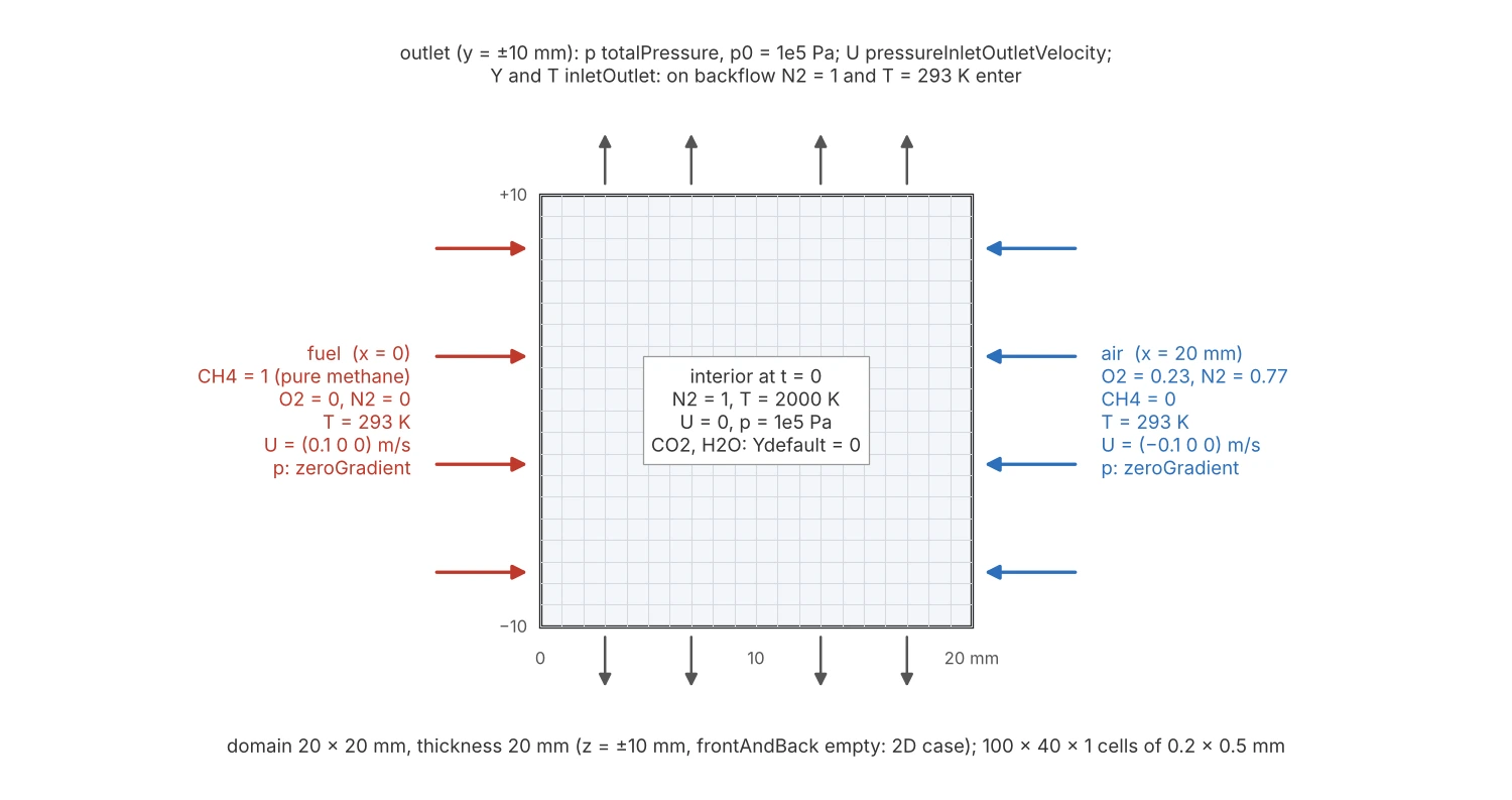
Geometry and boundary conditions read from blockMeshDict and the 0/ files of the tutorial (grid drawn every 5 cells in x and every 2 in y). Sketch, not a CFD result.
- The two jets have the same velocity, 0.1 m/s, but different densities (methane 0.659 kg/m³, air 1.184 kg/m³ at 293 K and 1 bar): the momentum flux ρU² of the air is 1.8 times that of the methane, so the stagnation plane is not at mid-domain but shifted towards the fuel inlet.
- With Zst = 0.0545 the stoichiometric surface lies where mixing has brought very little fuel, i.e. on the air side of the stagnation plane: the flame sits on the oxidiser side, as in all counterflow flames with undiluted fuel (Y. Tsuji, “Counterflow diffusion flames”, Progress in Energy and Combustion Science 8, 93–119, 1982, doi:10.1016/0360-1285(82)90015-6).
- The outlets are the two faces y = ±10 mm.
totalPressurewith p₀ = 10⁵ Pa andpressureInletOutletVelocityallow backflow; in that caseinletOutletlets pure nitrogen at 293 K in. Persistent backflow is a warning sign to check (section 9), because it brings into the domain a gas that does not exist in the physical problem. - The case is 2D: a single cell in z and the
frontAndBackfaces ofemptytype. Cells are rectangular, 0.2 mm in x and 0.5 mm in y: resolution is finer in the direction of the main gradients.
Deep dive · The thermophysical model, entry by entry
hePsiThermo: density is ρ = ψ·p with ψ = 1/(R·T) (compressibility), suitable for low-speed gases with large temperature changes; here pressure variations are negligible and ρ depends in practice on T and composition.coefficientWilkeMulticomponentMixture: species properties are computed separately and combined; mixture viscosity uses the rule of C. R. Wilke, “A viscosity equation for gas mixtures”, Journal of Chemical Physics 18, 517–519, 1950, doi:10.1063/1.1747673. It is more accurate, and more expensive, than a mass-weighted average of the coefficients.sutherland: μ = As·√T/(1 + Ts/T) (W. Sutherland, “The viscosity of gases and molecular force”, Philosophical Magazine 36, 507–531, 1893, doi:10.1080/14786449308620508); conductivity uses the Eucken correction, in the codekappa = mu*Cv*(1.32 + 1.77*R/Cv)(sutherlandTransportI.H).janaf: cp/R is a fourth-degree polynomial in T with two coefficient sets, below and aboveTcommon(1000 K); the sixth and seventh coefficients fix the reference enthalpy and entropy. Valid betweenTlow200 K andThigh5000 K (6000 K for methane). It is the NASA 7-coefficient format (B. J. McBride, M. J. Zehe, S. Gordon, NASA/TP-2002-211556, 2002).sensibleEnthalpy,perfectGas,specie: energy variable, equation of state and species data (molar mass).perfectGasis why the case cannot be reused for a liquid (section 15).
Practical tip · The tutorial variants in OpenFOAM 14 and when to use them
| Tutorial | Difference | Use |
|---|---|---|
counterFlowFlame2DLTS | same case, ddtSchemes localEuler (local time step), maxCo 1, maxDeltaT 1e-2, alphaTemp 0.05, 1000 iterations | reach the steady solution faster; intermediate times have no physical meaning |
counterFlowFlame2D_GRI | GRI-Mech 3.0, 53 species and 325 reactions; cpuLoad on, loadBalancer load balancing, Allrun-parallel with decomposePar -cellProc | detailed chemistry: CO, H₂, radicals, realistic temperature |
counterFlowFlame2D_GRI_TDAC | as GRI, with DAC dynamic reduction (tolerance 10⁻⁴) and ISAT tabulation (tolerance 3·10⁻³) | reduce the cost of detailed chemistry |
counterFlowFlame2DLTS_GRI_TDAC | both techniques together | steady state with detailed chemistry |
The LTS variant has the same reaction files, initial conditions, mesh and functions as the base case (checked with diff on the sources): for the A/B/C experiments at steady state it can replace it, applying the same prepare_cases.py with --source $FOAM_TUTORIALS/multicomponentFluid/counterFlowFlame2DLTS. References for the techniques: S. B. Pope, “Computationally efficient implementation of combustion chemistry using in situ adaptive tabulation”, Combustion Theory and Modelling 1, 41–63, 1997, doi:10.1080/713665229; F. Contino et al., “Coupling of in situ adaptive tabulation and dynamic adaptive chemistry: an effective method for solving combustion in engine simulations”, Proceedings of the Combustion Institute 33, 3057–3064, 2011, doi:10.1016/j.proci.2010.08.002.
5. The initial state: ignition matters
The official case specifies T = 293 K at both fuel and air inlets, while setting an initial internal temperature of 2000 K. This is a numerical ignition strategy for the reacting-flow configuration. It is not an experiment showing spontaneous reaction at room temperature.
The fuel boundary specifies pure methane (CH4 = 1), while the air boundary uses mass fractions O2 = 0.23 and N2 = 0.77. The initial methane and oxygen fields are zero within the domain. Check 0/N2, 0/Ydefault, and consistency of mass fractions before execution; the complete mixture composition must be physically consistent.
Deep dive · Boundary and initial compositions: the sum check, row by row
| Zone | CH₄ | O₂ | N₂ | CO₂, H₂O | Sum | T [K] |
|---|---|---|---|---|---|---|
fuel | 1 | 0 | 0 | 0 (Ydefault) | 1 | 293 |
air | 0 | 0.23 | 0.77 | 0 (Ydefault) | 1 | 293 |
| interior, t = 0 | 0 | 0 | 1 | 0 (Ydefault) | 1 | 2000 |
outlet, backflow | 0 | 0 | 1 | 0 (Ydefault) | 1 | 293 |
- The fuel inlet is pure methane (YCH4 = 1, YN2 = 0), not a methane-rich mixture: the guide has been corrected on this point.
- CO₂ and H₂O have no file in
0/: OpenFOAM builds their fields from0/Ydefault, with value 0 everywhere. A species added tothermo.compressibleGasreceives the same conditions with no new file needed. - The tutorial air is O₂ + N₂ by mass (0.23 + 0.77), without argon: the N₂/O₂ molar ratio is 3.83 instead of 3.76; for comparisons with experimental data use the composition of the experiment.
Why 2000 K in the interior. With the tutorial kinetics the chemical time at the stoichiometric composition is about 4·10⁹ s (127 years) at 293 K, 8 s at 500 K, 3 ms at 700 K and 0.3 ms at 800 K: mixing gases at room temperature would ignite nothing. The initial hot nitrogen provides the activation energy where the jets meet; then the flame sustains itself, because the heat of reaction keeps the mixing zone hot. The initial transient (displacement of the hot nitrogen, ignition, settling) is not physical and must be excluded from averages: this is why section 11 uses a final time window.
Practical tip · Changing the ignition or starting from a burning flame
- For an ignition sensitivity study change only the
internalFieldof0/Tin a new copy, for instance withfoamDictionary -entry internalField -set "uniform 1500" 0/T: below a certain temperature the flame does not ignite, and finding this threshold is a useful check of the kinetics. - To refine the mesh (section 14) without repeating the ignition transient: prepare the refined copy, run
blockMeshand initialise it withmapFields ../A_reference -consistent -sourceTime latestTime(from the new case folder); the mapped fields are written to the start time directory. - To start cases B and C from the burning solution of A, same procedure: the comparison between steady states does not change and the run is shorter; comparing transients, instead, requires the same initial condition for all.
6. Safe setup from Windows
Use Notepad++ to inspect and edit scripts and FileZilla/SFTP to transfer them to the Linux server. From PowerShell, connect with ssh username@server, source the OpenFOAM 14 environment and check foamVersion and $FOAM_TUTORIALS. VS Code is not needed.
Create new copies in a directory separate from the installed tutorials:
python3 scripts/prepare_cases.py "$HOME/cfd_guide18_cases"The script locates $FOAM_TUTORIALS/multicomponentFluid/counterFlowFlame2D, verifies expected files and rejects pre-existing case destinations. It does not edit official tutorials. If the installed mechanism differs from the expected Foundation 14 configuration, it stops rather than applying a blind text replacement.
Deep dive · Package script: prepare_cases.py, tested on the version 14 tutorial
#!/usr/bin/env python3
# SPDX-License-Identifier: GPL-3.0-or-later
"""Prepare isolated Arrhenius-sensitivity cases from OpenFOAM Foundation 14."""
import argparse
import os
from pathlib import Path
import re
import shutil
import sys

CASES = {"A_reference": 1.0, "B_half_A": 0.5, "C_double_A": 2.0}
A_OFFICIAL = 5.2e16
BASE_REL = Path("multicomponentFluid/counterFlowFlame2D")


def prepare(source: Path, destination: Path) -> None:
    if not source.is_dir():
        raise ValueError(f"Tutorial not found: {source}")
    needed = ["constant/reactions", "constant/chemistryProperties", "system/controlDict",
              "system/blockMeshDict", "0/CH4", "0/O2", "0/T"]
    for name in needed:
        if not (source / name).is_file():
            raise ValueError(f"Missing official case file: {name}")
    reference = (source / "constant/reactions").read_text(encoding="utf-8")
    pattern = re.compile(r"(?m)^(\s*A\s+)([\d.eE+-]+)(\s*;\s*)$")
    match = list(pattern.finditer(reference))
    if len(match) != 1:
        raise ValueError("Expected exactly one Arrhenius A entry in constant/reactions")
    actual = float(match[0].group(2))
    if abs(actual - A_OFFICIAL) / A_OFFICIAL > 1e-8:
        raise ValueError(f"Unexpected official A={actual:g}; inspect installed tutorial manually")
    if any((destination / n).exists() for n in CASES):
        raise FileExistsError("At least one destination case exists; no case was modified")
    destination.mkdir(parents=True, exist_ok=True)
    for name, factor in CASES.items():
        target = destination / name
        shutil.copytree(source, target, symlinks=False)
        reaction_path = target / "constant/reactions"
        replaced = pattern.sub(lambda m: m.group(1) + f"{actual*factor:.9e}" + m.group(3), reference, count=1)
        reaction_path.write_text(replaced, encoding="utf-8")
        (target / "GUIDE18_VARIANT.txt").write_text(
            "OpenFOAM Foundation 14 tutorial copy\n"
            f"Variant: {name}\nKinetic prefactor multiplier: {factor:g}\n"
            f"Original A: {actual:.9e}\nModified A: {actual*factor:.9e}\n"
            "This changes only constant/reactions. Case is NOT validated.\n", encoding="utf-8")
        print(f"CREATED: {target}")


def main() -> None:
    parser = argparse.ArgumentParser(description=__doc__)
    parser.add_argument("destination", type=Path, help="New parent folder for copies")
    parser.add_argument("--source", type=Path, help="Override official tutorial path")
    args = parser.parse_args()
    root = args.source or (Path(os.environ["FOAM_TUTORIALS"]) / BASE_REL if "FOAM_TUTORIALS" in os.environ else None)
    if root is None:
        parser.error("FOAM_TUTORIALS is missing: source your OpenFOAM-14 shell environment")
    try:
        prepare(root.resolve(), args.destination.expanduser().resolve())
    except (OSError, ValueError) as exc:
        print(f"ERROR: {exc}", file=sys.stderr)
        sys.exit(2)


if __name__ == "__main__":
main()- The tutorial is read and never modified; before copying, the script checks that seven expected files exist, that
constant/reactionscontains exactly oneA …;line and that its value is 5.2·10¹⁶ (relative tolerance 10⁻⁸): a different or already modified tutorial stops everything. - If even one of the three destination folders exists, no case is created or touched (
FileExistsError, exit 2). - The substitution rewrites the value in the
5.200000000e+16format: for A it is only a format change, as thediffwith the tutorial shows. TheGUIDE18_VARIANT.txtfile records factor and values; it is also the marker thatrun_case.shrequires. - With
--sourceone can point to another copy of the tutorial (for instance the LTS variant, section 4), provided it has the same files and the same A.
Test on the version 14 tutorial (with FOAM_TUTORIALS set as etc/bashrc does):
$ python3 scripts/prepare_cases.py "$HOME/cfd_guide18_cases"
CREATED: /home/user/cfd_guide18_cases/A_reference
CREATED: /home/user/cfd_guide18_cases/B_half_A
CREATED: /home/user/cfd_guide18_cases/C_double_A
[exit 0]
$ ls "$HOME/cfd_guide18_cases" "$HOME/cfd_guide18_cases/A_reference"
/home/user/cfd_guide18_cases:
A_reference
B_half_A
C_double_A

/home/user/cfd_guide18_cases/A_reference:
0
Allclean
GUIDE18_VARIANT.txt
constant
system
[exit 0]
$ cat "$HOME/cfd_guide18_cases/B_half_A/GUIDE18_VARIANT.txt"
OpenFOAM Foundation 14 tutorial copy
Variant: B_half_A
Kinetic prefactor multiplier: 0.5
Original A: 5.200000000e+16
Modified A: 2.600000000e+16
This changes only constant/reactions. Case is NOT validated.
[exit 0]
$ diff -r "$HOME/cfd_guide18_cases/A_reference" "$HOME/cfd_guide18_cases/B_half_A"
diff -r /home/user/cfd_guide18_cases/A_reference/GUIDE18_VARIANT.txt /home/user/cfd_guide18_cases/B_half_A/GUIDE18_VARIANT.txt
2,3c2,3
< Variant: A_reference
< Kinetic prefactor multiplier: 1
---
> Variant: B_half_A
> Kinetic prefactor multiplier: 0.5
5c5
< Modified A: 5.200000000e+16
---
> Modified A: 2.600000000e+16
diff -r /home/user/cfd_guide18_cases/A_reference/constant/reactions /home/user/cfd_guide18_cases/B_half_A/constant/reactions
25c25
<         A        5.200000000e+16;
---
>         A        2.600000000e+16;
[exit 1]
$ diff "$HOME/cfd_guide18_cases/A_reference/constant/reactions" "$HOME/cfd_guide18_cases/C_double_A/constant/reactions"
25c25
<         A        5.200000000e+16;
---
>         A        1.040000000e+17;
[exit 1]
$ diff "$FOAM_TUTORIALS/multicomponentFluid/counterFlowFlame2D/constant/reactions" "$HOME/cfd_guide18_cases/A_reference/constant/reactions"
25c25
<         A        5.2e16;
---
>         A        5.200000000e+16;
[exit 1]
$ python3 scripts/prepare_cases.py "$HOME/cfd_guide18_cases"
ERROR: At least one destination case exists; no case was modified
[exit 2]
Practical tip · The complete sequence on the server, with the balance monitors
The functions needed for the balances (sections 9 and 11) must be installed before the run, in never-started cases. Recommended sequence, from the folder containing the archive’s scripts/ and extra/:
source /opt/openfoam14/etc/bashrc      # path of your installation
foamVersion                            # OpenFOAM-14
python3 scripts/prepare_cases.py "$HOME/cfd_guide18_cases"
for c in A_reference B_half_A C_double_A; do
    python3 extra/add_monitors.py "$HOME/cfd_guide18_cases/$c"
done
python3 extra/reaction_thermo.py "$HOME/cfd_guide18_cases/A_reference"   # a-priori numbers
tmux new -s g18
bash scripts/run_case.sh "$HOME/cfd_guide18_cases/A_reference"
add_monitors.py checks that the case has never been started and that system/functions is the tutorial one; it keeps the original as system/functions.tutorial. It touches neither constant/ nor 0/, so it does not change the physics: A, B and C remain comparable. With FileZilla transfer the scripts/ and extra/ folders in binary or automatic mode; if a script edited on Windows gives errors such as $'\r': command not found, convert its line endings with sed -i 's/\r$//' scripts/run_case.sh (in Notepad++: Edit › EOL Conversion › Unix).
7. Three kinetic sensitivity experiments
| Experiment | Directory | Arrhenius prefactor | Aim |
|---|---|---|---|
| A | A_reference | 5.2e16 | official reference |
| B | B_half_A | 2.6e16 | reduced reaction-rate prefactor |
| C | C_double_A | 1.04e17 | increased reaction-rate prefactor |
Change only prefactor A in constant/reactions. Geometry, boundary conditions, transport and thermal models remain the same. Do not assume beforehand that the peak temperature or conversion will increase monotonically: nonlinear coupling can cause extinction, movement of the reaction zone or qualitatively different solutions.
Deep dive · What to expect from A, B and C: the Burke–Schumann limit and the structure of the reaction zone
When chemistry is much faster than transport (Da ≫ 1) fuel and oxidiser cannot coexist: they are consumed on a thin surface where Z = Zst, and temperature and composition depend only on Z (curve of section 3). This is the solution of S. P. Burke, T. E. W. Schumann, “Diffusion flames”, Industrial & Engineering Chemistry 20, 998–1004, 1928, doi:10.1021/ie50226a005. In this limit the total heat release is fixed by the diffusive flux of reactants towards the stoichiometric surface, i.e. by the flow field and diffusion, not by A.
With large but finite Da the reaction zone has its own thickness, with reactant leakage in both directions; the high-activation-energy asymptotic analysis of A. Liñán, “The asymptotic structure of counterflow diffusion flames for large activation energies”, Acta Astronautica 1, 1007–1039, 1974, doi:10.1016/0094-5765(74)90066-6, shows that in the diffusion-flame regime the relative thickness of the reaction zone decreases as Da−1/3 and that the flame extinguishes below a critical Damköhler number (S-curve). Applied to the three experiments:
| A | B (A/2) | C (2A) | |
|---|---|---|---|
| τchem at 2000 K | 2.6·10⁻⁸ s | 5.2·10⁻⁸ s | 1.3·10⁻⁸ s |
| Da = 1/(a·τ) | 3.8·10⁶ | 1.9·10⁶ | 7.7·10⁶ |
| relative reaction-zone thickness (∝ Da−1/3) | 1 | 1.26 | 0.79 |
| equivalent “kinetic” T change | 0 | −186 K | +186 K |
Expectations, to be checked with the run: peak temperature and integral heat release almost equal in the three cases (both limited by stoichiometry and mixing); higher Qdot peak and thinner reaction zone in C, the opposite in B; flame position almost unchanged, because it is tied to Z = Zst. If the results show large differences in peak temperature, before attributing them to the kinetics check time convergence (section 11) and the resolution of the reaction zone (section 14). For the detailed structure of counterflow methane flames: K. Seshadri, N. Peters, “Asymptotic structure and extinction of methane–air diffusion flames”, Combustion and Flame 73, 23–44, 1988, doi:10.1016/0010-2180(88)90051-X; for comparison with measurements, M. D. Smooke, I. K. Puri, K. Seshadri, “A comparison between numerical calculations and experimental measurements of the structure of a counterflow diffusion flame burning diluted methane in diluted air”, Symposium (International) on Combustion 21, 1783–1792, 1988, doi:10.1016/S0082-0784(88)80412-0.
Practical tip · Extending the campaign: other factors on A and the search for extinction
With factors 0.5 and 2 one stays far from extinction (Da ≈ 10⁶). To see the effect of kinetics on the heat release, A must be reduced by orders of magnitude. prepare_cases.py has fixed factors; for an additional variant copy a freshly prepared, never-run folder and change only A and the marker file:
cd "$HOME/cfd_guide18_cases"
cp -r A_reference D_A_div1e3                       # before A_reference is run
sed -i 's/^\(\s*A\s\+\)5\.200000000e+16;/\15.200000000e+13;/' D_A_div1e3/constant/reactions
grep -n "^ *A " D_A_div1e3/constant/reactions       # check: one line, new value
sed -i 's/^Variant: .*/Variant: D_A_div1e3/; s/^Kinetic prefactor multiplier: .*/Kinetic prefactor multiplier: 0.001/; s/^Modified A: .*/Modified A: 5.200000000e+13/' D_A_div1e3/GUIDE18_VARIANT.txt
bash scripts/run_case.sh "$HOME/cfd_guide18_cases/D_A_div1e3"
Proceeding by decades (10⁻¹, 10⁻², 10⁻³, …) one looks for the factor below which, after the transient, the peak temperature drops towards 293 K and volIntegrate(Qdot) towards zero. With a global mechanism the extinction found is a property of the model, not of real methane; the qualitative comparison with Liñán’s S-curve is still instructive.
8. Running simulations, logs and failure states
Run each case separately:
bash scripts/run_case.sh "$HOME/cfd_guide18_cases/A_reference"
bash scripts/run_case.sh "$HOME/cfd_guide18_cases/B_half_A"
bash scripts/run_case.sh "$HOME/cfd_guide18_cases/C_double_A"
The script performs blockMesh, checkMesh, then foamRun; it produces log.blockMesh, log.checkMesh and log.foamRun. Files status.running, status.completed or status.failed track execution. The script refuses a case with pre-existing status or log files, protecting previous calculations. For longer jobs use tmux (Guide 1).
Use FileZilla to download the logs first, then CSV data and images. There is no need to transfer every time directory when ParaView accesses the case through Linux pvserver.
Deep dive · Package script: run_case.sh and its safeguards
#!/usr/bin/env bash
# SPDX-License-Identifier: GPL-3.0-or-later
# Run one newly prepared OpenFOAM 14 case; never clean or overwrite old output.
set -Eeuo pipefail
if [[ $# -ne 1 ]]; then
  printf 'Usage: %s /path/to/case\n' "$0" >&2
  exit 2
fi
case_dir="$(realpath "$1")"
[[ -f "$case_dir/GUIDE18_VARIANT.txt" ]] || { echo 'Not a Guide 18 prepared case' >&2; exit 2; }
[[ -n "${WM_PROJECT_DIR:-}" ]] || { echo 'Source OpenFOAM environment first' >&2; exit 2; }
for tool in blockMesh checkMesh foamRun; do
  command -v "$tool" >/dev/null || { echo "Missing $tool" >&2; exit 2; }
done
if [[ -e "$case_dir/status.running" || -e "$case_dir/status.completed" || -e "$case_dir/status.failed" || -e "$case_dir/log.blockMesh" || -e "$case_dir/log.foamRun" ]]; then
  echo "Existing run/status detected; preserving all data: $case_dir" >&2
  exit 3
fi
cd "$case_dir"
printf 'RUNNING %s\n' "$case_dir"
printf '%s\n' "$(date -Is)" > status.running
trap 'rc=$?; if [[ $rc -ne 0 ]]; then printf "FAILED (exit=%s) %s\n" "$rc" "$(date -Is)" > status.failed; fi; rm -f status.running' EXIT
blockMesh > log.blockMesh 2>&1
checkMesh > log.checkMesh 2>&1
foamRun > log.foamRun 2>&1
printf 'COMPLETED %s\n' "$(date -Is)" > status.completed
printf 'Finished %s\n' "$case_dir"
set -Eeuo pipefail: the first failing command stops the script; thetraponEXITwritesstatus.failedwith the exit code and always removesstatus.running.- It refuses folders without
GUIDE18_VARIANT.txt, an OpenFOAM environment not loaded (emptyWM_PROJECT_DIR), missing commands and cases with existing logs or status (exit 3): no result is overwritten. - Two checks to do by hand after the run, because the script does not do them: that
log.checkMeshcontains “Mesh OK.” and not “Failed … mesh checks” (in the source of checkMesh.C the program always ends withreturn 0, even when checks fail, soset -edoes not catch it) and thatlog.foamRunends with the “End” line:grep -E "Mesh OK|Failed" log.checkMesh; tail -n 2 log.foamRun.
Test with the OpenFOAM commands replaced by placeholders that write short logs (same sequence of files and checks; in C the foamRun placeholder exits with an error to test the failure branch):
$ bash scripts/run_case.sh "$HOME/cfd_guide18_cases/A_reference"
RUNNING /home/user/cfd_guide18_cases/A_reference
Finished /home/user/cfd_guide18_cases/A_reference
[exit 0]
$ ls "$HOME/cfd_guide18_cases/A_reference"
0
Allclean
GUIDE18_VARIANT.txt
constant
log.blockMesh
log.checkMesh
log.foamRun
status.completed
system
[exit 0]
$ cat "$HOME/cfd_guide18_cases/A_reference/status.completed"
COMPLETED 2026-10-31T15:00:28+01:00
[exit 0]
$ bash scripts/run_case.sh "$HOME/cfd_guide18_cases/A_reference"
Existing run/status detected; preserving all data: /home/user/cfd_guide18_cases/A_reference
[exit 3]
$ PATH=/usr/bin:/bin bash scripts/run_case.sh "$HOME/cfd_guide18_cases/B_half_A"
Missing blockMesh
[exit 2]
$ ls "$HOME/cfd_guide18_cases/B_half_A"
0
Allclean
GUIDE18_VARIANT.txt
constant
system
[exit 0]
Practical tip · Following the run: log, time step and duration
tail -f log.foamRun                         # live (Ctrl+C stops only tail)
grep "^deltaT" log.foamRun | tail -n 3        # current time step
grep "Courant Number" log.foamRun | tail -n 3
grep -c "^Time = " log.foamRun                # steps done
foamLog log.foamRun                           # logs/ folder: one file per quantity
ls logs/
tmux attach -t g18 # back to the session after disconnecting- The initial step is 10⁻⁶ s and
adjustTimeStep yesgrows it up to themaxCo 0.4limit. With 0.2 mm cells and velocities of the order of 0.1–1 m/s (thermal expansion accelerates the gas in the hot zone) the limiting step is of the order of 10⁻⁴ s: a few thousand steps for 0.5 s. - For every step the log reports the solution of O2, H2O, CH4, CO2 (not N2, the balance species), of the enthalpy
hand of pressure; with the section 9 monitors also the function lines. - Run time depends mainly on chemistry integration in the hot cells: with a one-reaction mechanism and 4000 cells it stays modest; with GRI-Mech (53 species) it grows by orders of magnitude, and that is where TDAC and parallel runs are needed.
9. Diagnostics: flow stability, chemistry and fields
Monitor residuals, Time, actual step size, Courant number, thermophysical warnings and chemistry integration behavior. A program that exits normally is not necessarily converged or physically correct. Check Y_i ≥ 0, plausible fractions, physically plausible pressure and temperature and sensitivity to mesh and time discretization.
The tutorial has #includeFunc Qdot, linked to the volumetric heat-release rate. Confirm which field is actually written by the installed version and verify its dimensions and sign before volume integration. In OpenFOAM 14 the field is named Qdot, is expressed in W/m³, is positive for exothermic reactions and, with the tutorial configuration, is computed and written only at write times (details in the boxes of this section). A local peak in Qdot is not total power.
Deep dive · Qdot in the code: definition, units, sign and when it is computed
The field is built by Standard_chemistryModel.C:
tmp<volScalarField> tQdot
(
    volScalarField::New
    (
        "Qdot",
        this->mesh_,
        dimensionedScalar(dimEnergy/dimVolume/dimTime, 0)
    )
);
...
forAll(Yvf_, i)
{
    ...
        const scalar hi = specieThermos_[i].hf();
        Qdot[celli] -= hi*RR_[i][celli];
}- Qdot = −Σ hf,i·ω̇i, with hf the formation enthalpy at 298.15 K [J/kg] and ω̇ the production rate [kg/(m³·s)]: the unit is W/m³ and the value is positive for an exothermic reaction. It is the same term that appears on the right-hand side of the sensible enthalpy equation (section 2).
- For the tutorial global reaction Qdot = 50.03 MJ/kg × local methane consumption rate: this is the check used by
species_balance.py(section 11). - The
Qdotfunction (libreactionModels.so) hasexecuteControl writeTimeandwriteControl writeTime: the field is computed and written only at write times (every 0.05 s). That is enough for maps in ParaView, not for following the integrated heat release over time: this is why the monitors in the next box compute it at every step. Allcleanalso removes0/Qdot, which is created if the function is executed on the initial time (for example withfoamPostProcess).- Upper bound for checking: ∫Qdot dV ≤ 136.6 W over the whole mesh (section 1). A higher value indicates a balance error or a transient not yet over (the initial hot nitrogen contains energy that does not come from Qdot).
Deep dive · Additional script: add_monitors.py and the functions_guide18 file for the balances
The script replaces system/functions of a new case with the file below (generated from the species of thermo.compressibleGas and identical to extra/functions_guide18 in the archive). Each entry uses the standard configurations of etc/caseDicts/functions with arguments, the same syntax as the multicomponentFluid/membrane tutorial:
/*--------------------------------*- C++ -*----------------------------------*\
  Guide 18 - balance monitors for counterFlowFlame2D (OpenFOAM 14)
  Generated by add_monitors.py; the tutorial original is system/functions.tutorial
\*---------------------------------------------------------------------------*/
FoamFile
{
    format      ascii;
    class       dictionary;
    location    "system";
    object      functions;
}
// * * * * * * * * * * * * * * * * * * * * * * * * * * * * * * * * * * * * * //

// Heat release rate [W/m3]: computed at every step (tutorial default: write times only),
// the field is still written only at write times.
#includeFunc Qdot(executeControl=timeStep)

// Total specie flux (advective + diffusive) on every face [kg/s].
// schemesField=Yi_h: use the div(phi,Yi_h) scheme of the species equations.
#includeFunc specieFlux(O2,  schemesField=Yi_h, executeControl=timeStep)
#includeFunc specieFlux(H2O, schemesField=Yi_h, executeControl=timeStep)
#includeFunc specieFlux(CH4, schemesField=Yi_h, executeControl=timeStep)
#includeFunc specieFlux(CO2, schemesField=Yi_h, executeControl=timeStep)
#includeFunc specieFlux(N2,  schemesField=Yi_h, executeControl=timeStep)

// Patch sums (outward normal: negative = entering the domain) [kg/s].
#includeFunc patchFlux(name=fuelFlux, patch=fuel, phi, specieFlux(O2), specieFlux(H2O), specieFlux(CH4), specieFlux(CO2), specieFlux(N2))
#includeFunc patchFlux(name=airFlux, patch=air, phi, specieFlux(O2), specieFlux(H2O), specieFlux(CH4), specieFlux(CO2), specieFlux(N2))
#includeFunc patchFlux(name=outletFlux, patch=outlet, phi, specieFlux(O2), specieFlux(H2O), specieFlux(CH4), specieFlux(CO2), specieFlux(N2))

// Mass of every specie in the domain [kg] and integral heat release rate [W].
#includeFunc volIntegrate(name=specieMass, weightField=rho, O2, H2O, CH4, CO2, N2)
#includeFunc volIntegrate(name=heatRelease, Qdot)

// Volume-averaged rate of every reaction [kmol/m3/s] (independent check:
// rate x mesh volume = kmol/s of reaction).
#includeFunc reactionRates

// Maximum temperature and its position.
#includeFunc cellMax(name=Tmax, T)

// ************************************************************************* //| Function | What it writes | File and columns |
|---|---|---|
Qdot(executeControl=timeStep) | the Qdot field at every step (written to disk only at write times) | — |
specieFlux(Y, schemesField=Yi_h, …) | total flux (convective with the species scheme + diffusive) of Y on every face, field specieFlux(Y) [kg/s] | — |
patchFlux(name=fuelFlux, …) | sums over the patch faces | postProcessing/fuelFlux/0/surfaceFieldValue.dat: sum(phi), sum(specieFlux(O2)), … |
volIntegrate(name=specieMass, weightField=rho, …) | mass of every species in the domain, ∫ρY dV [kg] | specieMass/0/volFieldValue.dat: volIntegrate(rho,O2), … |
volIntegrate(name=heatRelease, Qdot) | heat release rate ∫Qdot dV [W] | heatRelease/0/volFieldValue.dat: volIntegrate(Qdot) |
reactionRates | volume-averaged rate of every reaction [kmol/(m³·s)]; × 8·10⁻⁶ m³ (mesh volume) = kmol/s of methane consumed | postProcessing/reactionRates/0/ |
cellMax(name=Tmax, T) | maximum temperature, position and cell | Tmax/0/volFieldValue.dat: max(T), location, cell |
Why specieFlux and not phi times Y: at the inlets diffusion is not negligible (cell Péclet close to 1 at 293 K, section 2). With YCH4 = 1 imposed on the fuel patch and nitrogen and products present inside, part of the products diffuses out through the inlet and methane enters by convection and diffusion: ρ·u·Y under- or over-estimates the true flux. The column names are those written by the code (writeFileHeader of volFieldValue.C and surfaceFieldValue.C).
#!/usr/bin/env python3
"""Install the Guide 18 balance monitors in a NEW counterFlowFlame2D copy.

The tutorial system/functions contains only '#includeFunc Qdot', which
computes the heat release rate field at write times only. This script
replaces it (the original is kept as system/functions.tutorial) with a
functions file that, at every time step, writes:

  * the total (advective + diffusive) flux of every specie through every
    inlet/outlet patch (specieFlux + patchFlux), together with sum(phi);
  * the mass of every specie in the domain (volIntegrate weighted by rho);
  * the volume integral of Qdot, the volume-averaged rate of every reaction
    (reactionRates) and the maximum temperature.

These are exactly the quantities needed by species_balance.py.
The case must not have been started: logs, status files, time directories
other than 0 or postProcessing make the script stop without changes.

Usage:  python3 add_monitors.py CASE_DIR [--patches fuel,air,outlet] [--print]
"""
import argparse, os, re, sys


def species(case):
    t = open(os.path.join(case, 'constant', 'thermo.compressibleGas'), encoding='utf-8').read()
    t = re.sub(r'//[^\n]*', '', re.sub(r'/\*.*?\*/', '', t, flags=re.S))
    return re.search(r'species\s*\(([^)]*)\)', t).group(1).split()


def functions_text(sp, patches):
    w = max(len(s) for s in sp)
    flux = ', '.join(f'specieFlux({s})' for s in sp)
    L = ['/*--------------------------------*- C++ -*----------------------------------*\\',
         '  Guide 18 - balance monitors for counterFlowFlame2D (OpenFOAM 14)',
         '  Generated by add_monitors.py; the tutorial original is system/functions.tutorial',
         '\\*---------------------------------------------------------------------------*/',
         'FoamFile', '{', '    format      ascii;', '    class       dictionary;', '    location    "system";',
         '    object      functions;', '}',
         '// * * * * * * * * * * * * * * * * * * * * * * * * * * * * * * * * * * * * * //', '',
         '// Heat release rate [W/m3]: computed at every step (tutorial default: write times only),',
         '// the field is still written only at write times.',
         '#includeFunc Qdot(executeControl=timeStep)', '',
         '// Total specie flux (advective + diffusive) on every face [kg/s].',
         '// schemesField=Yi_h: use the div(phi,Yi_h) scheme of the species equations.']
    for s in sp:
        L.append(f'#includeFunc specieFlux({s},{" " * (w - len(s))} schemesField=Yi_h, executeControl=timeStep)')
    L += ['', '// Patch sums (outward normal: negative = entering the domain) [kg/s].']
    for p in patches:
        L.append(f'#includeFunc patchFlux(name={p}Flux, patch={p}, phi, {flux})')
    L += ['', '// Mass of every specie in the domain [kg] and integral heat release rate [W].',
          '#includeFunc volIntegrate(name=specieMass, weightField=rho, ' + ', '.join(sp) + ')',
          '#includeFunc volIntegrate(name=heatRelease, Qdot)', '',
          '// Volume-averaged rate of every reaction [kmol/m3/s] (independent check:',
          '// rate x mesh volume = kmol/s of reaction).',
          '#includeFunc reactionRates', '',
          '// Maximum temperature and its position.',
          '#includeFunc cellMax(name=Tmax, T)', '',
          '// ************************************************************************* //']
    return '\n'.join(L) + '\n'


def started(case):
    bad = [f for f in os.listdir(case) if f.startswith(('log.', 'status.')) or f in ('postProcessing', 'processor0')]
    for f in os.listdir(case):
        try:
            if float(f) != 0 and os.path.isdir(os.path.join(case, f)):
                bad.append(f)
        except ValueError:
            pass
    if os.path.isdir(os.path.join(case, 'constant', 'polyMesh')):
        bad.append('constant/polyMesh')
    return sorted(bad)


def main():
    ap = argparse.ArgumentParser(description='Install the Guide 18 balance monitors in a new case copy.')
    ap.add_argument('case')
    ap.add_argument('--patches', default='fuel,air,outlet')
    ap.add_argument('--print', action='store_true', help='print the functions file and change nothing')
    a = ap.parse_args()
    case = os.path.abspath(a.case)
    fn = os.path.join(case, 'system', 'functions')
    if not os.path.isfile(fn) or not os.path.isfile(os.path.join(case, 'constant', 'thermo.compressibleGas')):
        sys.exit('not a counterFlowFlame2D-type case: ' + case)
    text = functions_text(species(case), a.patches.split(','))
    if a.print:
        sys.stdout.write(text)
        return
    bad = started(case)
    if bad:
        sys.exit('case already started or meshed (' + ', '.join(bad) + '): use a new copy, nothing changed')
    orig = open(fn, encoding='utf-8').read()
    if 'Guide 18 - balance monitors' in orig:
        sys.exit('Guide 18 monitors already installed in ' + a.case + ': nothing changed')
    body = re.sub(r'//[^\n]*', '', re.sub(r'/\*.*?\*/', '', orig, flags=re.S))
    body = re.sub(r'FoamFile\s*\{[^}]*\}', '', body).split()
    if body != ['#includeFunc', 'Qdot']:
        sys.exit('system/functions differs from the tutorial (' + ' '.join(body)[:80] + '): nothing changed')
    bak = fn + '.tutorial'
    if os.path.exists(bak):
        sys.exit(bak + ' already exists: nothing changed')
    os.rename(fn, bak)
    with open(fn, 'w', encoding='utf-8') as f:
        f.write(text)
    print('installed', os.path.join(a.case, 'system', 'functions'), '(original kept as functions.tutorial)')


if __name__ == '__main__':
    main()
Test on the version 14 tutorial (new copy, already started copy, copy with a customised functions):
$ python3 add_monitors.py A_new
installed A_new/system/functions (original kept as functions.tutorial)
exit 0
$ ls A_new/system
blockMeshDict
controlDict
functions
functions.tutorial
fvSchemes
fvSolution
$ diff A_new/system/functions functions_guide18
identical
$ python3 add_monitors.py A_new   # second time
Guide 18 monitors already installed in A_new: nothing changed
exit 1
$ python3 add_monitors.py A_started
case already started or meshed (0.05, log.blockMesh): use a new copy, nothing changed
exit 1
$ python3 add_monitors.py A_custom
system/functions differs from the tutorial (#includeFunc Qdot #includeFunc mag(U)): nothing changed
exit 1
Practical tip · Plausibility checks on the fields, with the commands
cd "$HOME/cfd_guide18_cases/A_reference"
foamPostProcess -func "cellMin(CH4, O2, CO2, H2O, N2)" -latestTime   # must be >= 0 (round-off aside)
foamPostProcess -func "cellMax(T)" -latestTime                      # <= 2305 K with this mechanism
foamPostProcess -func "patchFlowRate(patch=outlet)" -latestTime     # > 0: net outflow
foamListTimes- Negative mass fractions beyond round-off indicate an unbounded convection scheme or too large a step; the tutorial uses
limitedLinear 1, which keeps them in check. - A peak temperature above the 2305 K adiabatic temperature is not physical with this mechanism: after the transient, it indicates an energy conservation error.
- Backflow at the outlets: in ParaView colour the
outletpatch by the y component of U; persistent inflow zones bring in cold nitrogen (section 4) and spoil the balances. - For a chemistry-driven time step OpenFOAM 14 offers the
adjustTimeStepToChemistryfunction (“Adjusts the time step to a chemistry model’s bulk chemical time scales”): useful in ignition transients, to be tried as a numerical variant.
10. Post-processing with ParaView on Windows
Connect to the Linux pvserver as described in Guide 3. Open the case and select CH4, O2, CO2, H2O, T, U and Qdot where available. The case is two-dimensional (a single cell in z, frontAndBack faces of type empty): the fields are viewed directly in the x–y plane, with no need for a Slice. Use identical color limits across the three cases, matching physical time and geometric location. Use Plot Over Line on the same line and Save Data to export profiles in CSV format.
For the provided script, rename CSV columns to x_m,CH4,O2,CO2,H2O,T_K using metres and numeric values in the stated units. Actual ParaView headers may differ; renaming the headers must not modify numerical values.
python inspect_profiles.py A_profile.csv B_profile.csv C_profile.csv --output summary_guide18.csvThe script records peak temperature, its location and species-fraction ranges. It does not infer chemical conversion from a single line profile, since that would not be physically justified.
Deep dive · Additional script: paraview_profile.py, from the ParaView export to the guide format with the mixture fraction
ParaView’s Plot Over Line → File › Save Data (CSV) export writes columns such as "CH4","CO2",…,"T","U:0",…,"vtkValidPointMask","arc_length","Points:0",…. The script copies the values without changing them, renames the columns to the x_m,CH4,O2,CO2,H2O,T_K format required by inspect_profiles.py, drops points outside the mesh (vtkValidPointMask = 0) and adds N₂, Qdot (if present), the sum of mass fractions and the Bilger mixture fraction (section 1). In the summary: position of the temperature peak, crossing of Zst, Qdot peak and full width at half maximum, line integral of Qdot.
#!/usr/bin/env python3
"""Convert a ParaView 'Plot Over Line' CSV of counterFlowFlame2D into the
x_m,CH4,O2,CO2,H2O,T_K format of inspect_profiles.py and analyse it.

ParaView (File > Save Data, CSV) writes columns such as
  "CH4","CO2","H2O","N2","O2","Qdot","T","U:0","U:1","U:2","p",
  "vtkValidPointMask","arc_length","Points:0","Points:1","Points:2"
The values are copied without changes; only the header is renamed and the
points outside the mesh (vtkValidPointMask = 0) are dropped. Added columns:

  N2, Qdot_W_m3 (if present), sumY (sum of the mass fractions),
  Z_Bilger: Bilger mixture fraction from the C, H, O element mass fractions,
            0 in the air stream and 1 in the fuel stream.

The summary gives the position of the stoichiometric surface Z = Z_st,
of the temperature peak and of the Qdot peak, and the Qdot full width at
half maximum. With unity Lewis number (the tutorial default,
unityLewisFourier) Z_Bilger is a conserved scalar.

Usage:
  python3 paraview_profile.py plot_A.csv --output A_profile.csv
        [--coord Points:0] [--fuel-Y 1] [--air-O2 0.23] [--air-N2 0.77]
"""
import argparse, csv, math, os, sys

W = {'C': 12.011, 'H': 1.008, 'O': 15.999, 'N': 14.007}
SP = {'CH4': {'C': 1, 'H': 4}, 'O2': {'O': 2}, 'CO2': {'C': 1, 'O': 2}, 'H2O': {'H': 2, 'O': 1}, 'N2': {'N': 2}}
MW = {'CH4': 16.0428, 'O2': 31.9988, 'CO2': 44.01, 'H2O': 18.0153, 'N2': 28.0134}   # thermo.compressibleGas


def beta(Y):
    """Bilger coupling function 2 Z_C/W_C + Z_H/(2 W_H) - Z_O/W_O from the specie mass fractions."""
    Z = {e: 0.0 for e in W}
    for s, comp in SP.items():
        for e, n in comp.items():
            Z[e] += Y.get(s, 0.0) * n * W[e] / MW[s]
    return 2 * Z['C'] / W['C'] + Z['H'] / (2 * W['H']) - Z['O'] / W['O']


def crossing(x, f, level):
    out = []
    for i in range(len(x) - 1):
        a, b = f[i] - level, f[i + 1] - level
        if a == 0:
            out.append(x[i])
        elif a * b < 0:
            out.append(x[i] + (x[i + 1] - x[i]) * a / (a - b))
    return out


def main():
    ap = argparse.ArgumentParser(description='ParaView Plot Over Line CSV -> Guide 18 profile CSV with mixture fraction.')
    ap.add_argument('csv')
    ap.add_argument('--output', required=True)
    ap.add_argument('--coord', default='Points:0', help='column used as x_m (Points:0, Points:1, arc_length)')
    ap.add_argument('--fuel-Y', type=float, default=1.0, help='CH4 mass fraction of the fuel stream')
    ap.add_argument('--air-O2', type=float, default=0.23)
    ap.add_argument('--air-N2', type=float, default=0.77)
    a = ap.parse_args()
    if os.path.exists(a.output):
        sys.exit('output exists and will not be overwritten: ' + a.output)
    with open(a.csv, newline='', encoding='utf-8-sig') as f:
        rd = csv.DictReader(f)
        cols = rd.fieldnames or []
        need = [a.coord, 'CH4', 'O2', 'CO2', 'H2O', 'T']
        miss = [c for c in need if c not in cols]
        if miss:
            sys.exit('missing columns in the ParaView CSV: ' + ', '.join(miss) + '\nfound: ' + ', '.join(cols))
        rows = []
        for i, r in enumerate(rd, start=2):
            if 'vtkValidPointMask' in r and float(r['vtkValidPointMask']) == 0:
                continue
            try:
                rows.append({k: float(r[k]) for k in cols if r.get(k, '') != ''})
            except ValueError:
                sys.exit(f'non-numeric value at line {i}')
    if len(rows) < 3:
        sys.exit('fewer than three valid points')
    rows.sort(key=lambda r: r[a.coord])
    b_fuel = beta({'CH4': a.fuel_Y, 'N2': 1 - a.fuel_Y})
    b_air = beta({'O2': a.air_O2, 'N2': a.air_N2})
    s = 2 * MW['O2'] / MW['CH4']
    Zst = a.air_O2 / (s * a.fuel_Y + a.air_O2)
    has_q = 'Qdot' in rows[0]
    has_n2 = 'N2' in rows[0]
    out = []
    for r in rows:
        Y = {k: r[k] for k in SP if k in r}
        if not has_n2:
            Y['N2'] = 1 - sum(Y.values())
        Zb = (beta(Y) - b_air) / (b_fuel - b_air)
        o = dict(x_m=r[a.coord], CH4=r['CH4'], O2=r['O2'], CO2=r['CO2'], H2O=r['H2O'], T_K=r['T'], N2=Y['N2'])
        if has_q:
            o['Qdot_W_m3'] = r['Qdot']
        o['sumY'] = sum(Y.values())
        o['Z_Bilger'] = Zb
        out.append(o)
    with open(a.output, 'x', newline='', encoding='utf-8') as f:
        w = csv.DictWriter(f, fieldnames=list(out[0]))
        w.writeheader()
        for o in out:
            w.writerow({k: f'{v:.7g}' for k, v in o.items()})
    x = [o['x_m'] for o in out]
    T = [o['T_K'] for o in out]
    Z = [o['Z_Bilger'] for o in out]
    print(f'{len(out)} points from {a.csv} written to {a.output} (coordinate {a.coord}, {x[0]:g} to {x[-1]:g} m)')
    print(f'sum of mass fractions: min {min(o["sumY"] for o in out):.6f}, max {max(o["sumY"] for o in out):.6f}')
    print(f'Z_Bilger range {min(Z):.4f} - {max(Z):.4f} (stream values: fuel 1, air 0)')
    ip = max(range(len(T)), key=T.__getitem__)
    print(f'T peak {T[ip]:.1f} K at x = {x[ip]:.5f} m, Z_Bilger = {Z[ip]:.4f}')
    zs = crossing(x, Z, Zst)
    print(f'Z_st = {Zst:.4f} crossed at x = ' + (', '.join(f'{v:.5f}' for v in zs) + ' m' if zs else 'nowhere on the line'))
    if zs:
        print(f'distance between the T peak and the nearest Z_st crossing: {1e3 * min(abs(v - x[ip]) for v in zs):.3f} mm')
    if has_q:
        q = [o['Qdot_W_m3'] for o in out]
        iq = max(range(len(q)), key=q.__getitem__)
        half = crossing(x, q, q[iq] / 2)
        print(f'Qdot peak {q[iq]:.4e} W/m3 at x = {x[iq]:.5f} m', end='')
        left = [v for v in half if v < x[iq]]
        right = [v for v in half if v > x[iq]]
        if left and right:
            print(f', full width at half maximum {1e3 * (min(right) - max(left)):.3f} mm')
        else:
            print(' (half-maximum width not bounded on this line)')
        integ = sum(0.5 * (q[i] + q[i + 1]) * (x[i + 1] - x[i]) for i in range(len(x) - 1))
        print(f'line integral of Qdot: {integ:.4e} W/m2 (heat release per unit flame area along this line)')
    print('No conversion is inferred from a line profile: use species_balance.py for balances.')


if __name__ == '__main__':
    main()
To test it without a run, make_synthetic_paraview.py writes a CSV in the ParaView format with an imposed mixture-fraction profile (error function) and the Burke–Schumann state of the T(Z) curve: synthetic data, not OpenFOAM results.
#!/usr/bin/env python3
"""SYNTHETIC ParaView-style 'Plot Over Line' CSV to test paraview_profile.py.

NOT an OpenFOAM result. The mixture fraction follows an imposed error
function profile Z(x) = erfc((x - x0)/delta)/2 between the fuel inlet
(x = 0, Z = 1) and the air inlet (x = L, Z = 0); composition and
temperature are the Burke-Schumann (infinitely fast chemistry) state of
the T(Z) table written by reaction_thermo.py --csv; Qdot is a Gaussian
centred on the stoichiometric surface. Header and layout imitate
File > Save Data in ParaView; two points are flagged outside the mesh.

Usage: python3 make_synthetic_paraview.py tz.csv OUT.csv [--x0 0.0125] [--delta 0.004]
"""
import argparse, csv, math, os, sys


def main():
    ap = argparse.ArgumentParser()
    ap.add_argument('tz')
    ap.add_argument('out')
    ap.add_argument('--x0', type=float, default=0.0125)
    ap.add_argument('--delta', type=float, default=0.004)
    ap.add_argument('--length', type=float, default=0.02)
    ap.add_argument('--n', type=int, default=201)
    a = ap.parse_args()
    if os.path.exists(a.out):
        sys.exit('output exists: ' + a.out)
    tab = list(csv.DictReader(open(a.tz, encoding='utf-8')))
    Zt = [float(r['Z']) for r in tab]

    def interp(Z, key):
        for i in range(len(Zt) - 1):
            if Zt[i] <= Z <= Zt[i + 1]:
                f = (Z - Zt[i]) / (Zt[i + 1] - Zt[i])
                return float(tab[i][key]) * (1 - f) + float(tab[i + 1][key]) * f
        return float(tab[-1][key])

    Zst = 0.23 / (2 * 31.9988 / 16.0428 + 0.23)
    # position of Z_st on the erfc profile (bisection)
    lo, hi = 0.0, a.length
    for _ in range(80):
        mid = 0.5 * (lo + hi)
        if 0.5 * math.erfc((mid - a.x0) / a.delta) > Zst:
            lo = mid
        else:
            hi = mid
    xst = 0.5 * (lo + hi)
    hdr = ['CH4', 'CO2', 'H2O', 'N2', 'O2', 'Qdot', 'T', 'U:0', 'U:1', 'U:2', 'p', 'vtkValidPointMask', 'arc_length',
           'Points:0', 'Points:1', 'Points:2']
    with open(a.out, 'w', newline='', encoding='utf-8') as f:
        f.write(','.join(f'"{h}"' for h in hdr) + '\n')
        for i in range(a.n + 2):
            x = -a.length / (a.n - 1) + i * a.length / (a.n - 1)     # first and last points fall outside the mesh
            inside = 0 <= x <= a.length + 1e-12
            xc = min(max(x, 0.0), a.length)
            Z = 0.5 * math.erfc((xc - a.x0) / a.delta)
            Y = {k: interp(Z, 'Y_' + k) for k in ('CH4', 'O2', 'CO2', 'H2O')}
            Y['N2'] = 1 - sum(Y.values())
            T = interp(Z, 'T_burnt_K')
            q = 2.0e6 * math.exp(-((xc - xst) / 0.0006) ** 2)
            u = 0.1 * (1 - 2 * xc / a.length)
            vals = [Y['CH4'], Y['CO2'], Y['H2O'], Y['N2'], Y['O2'], q, T, u, 0, 0, 1e5, 1 if inside else 0,
                    x + a.length / (a.n - 1), x, 0, 0]
            f.write(','.join(f'{v:.7g}' for v in vals) + '\n')
    print(f'SYNTHETIC ParaView CSV written: {a.out} ({a.n} points inside, Z_st at x = {xst:.5f} m)')


if __name__ == '__main__':
    main()
# tz.csv was written by: python3 reaction_thermo.py A_reference --csv tz.csv
$ python3 make_synthetic_paraview.py tz.csv plot_A_SYNTHETIC.csv
SYNTHETIC ParaView CSV written: plot_A_SYNTHETIC.csv (201 points inside, Z_st at x = 0.01703 m)
$ head -3 plot_A_SYNTHETIC.csv
"CH4","CO2","H2O","N2","O2","Qdot","T","U:0","U:1","U:2","p","vtkValidPointMask","arc_length","Points:0","Points:1","Points:2"
0.9999948,7.826674e-07,6.407631e-07,3.809963e-06,0,0,293.0064,0.1,0,0,100000,0,0,-0.0001,0,0
0.9999948,7.826674e-07,6.407631e-07,3.809963e-06,0,0,293.0064,0.1,0,0,100000,1,0.0001,0,0,0
$ python3 paraview_profile.py plot_A_SYNTHETIC.csv --output A_profile.csv
201 points from plot_A_SYNTHETIC.csv written to A_profile.csv (coordinate Points:0, 0 to 0.02 m)
sum of mass fractions: min 1.000000, max 1.000000
Z_Bilger range 0.0040 - 1.0000 (stream values: fuel 1, air 0)
T peak 2295.8 K at x = 0.01700 m, Z_Bilger = 0.0558
Z_st = 0.0545 crossed at x = 0.01703 m
distance between the T peak and the nearest Z_st crossing: 0.033 mm
Qdot peak 1.9940e+06 W/m3 at x = 0.01700 m, full width at half maximum 1.003 mm
line integral of Qdot: 2.1269e+03 W/m2 (heat release per unit flame area along this line)
No conversion is inferred from a line profile: use species_balance.py for balances.
exit 0
$ head -3 A_profile.csv
x_m,CH4,O2,CO2,H2O,T_K,N2,Qdot_W_m3,sumY,Z_Bilger
0,0.9999948,0,7.826674e-07,6.407631e-07,293.0064,3.809963e-06,0,1,0.9999951
0.0001,0.9999938,0,9.212154e-07,7.541912e-07,293.0076,4.484403e-06,0,1,0.9999941
$ python3 paraview_profile.py plot_A_SYNTHETIC.csv --output A_profile.csv # again
output exists and will not be overwritten: A_profile.csv
exit 1
$ python3 inspect_profiles.py A_profile.csv --output summary_guide18_pv.csv
Wrote summary_guide18_pv.csv; no species conversion inferred from a line profile
source,points,T_peak_K,x_at_T_peak_m,CH4_min,CH4_max,CO2_max
A_profile.csv,201,2295.813,0.017,0.0,0.9999948,0.1493405The check succeeds as expected: the mixture fraction rebuilt from the elements is 1 at the methane inlet, the sum of mass fractions is 1 and the temperature peak falls on the Zst crossing (0.03 mm apart, the point spacing is 0.1 mm). On a real profile, a distance of many cells between the T peak and Zst indicates that the flame is far from the fast-chemistry limit or that the solution is not yet steady.
Practical tip · Plot Over Line in ParaView: reproducible settings for A, B and C
- Open each case with an empty
A_reference.foamfile (touch A_reference.foamin the case folder) and the OpenFOAM reader; inMesh RegionskeepinternalMesh. - The case is 2D: no
Sliceis needed; the front view (z axis towards the viewer) already shows the fields. If a section is wanted anyway, use a plane normal to z at z = 0. - Recommended line: the jet axis, from
(0 0 0)to(0.02 0 0), withResolution200 (two points per cell in x). It is the line through the stagnation point that crosses the flame perpendicularly. - Same time for the three cases (the last one, 0.5 s, if the section 11 monitors are steady), same line, same resolution; in
Save Datadisable writing all time steps and raise the precision to 8 digits. - Command for each file:
python3 extra/paraview_profile.py plot_A.csv --output A_profile.csv; thenpython scripts/inspect_profiles.py A_profile.csv B_profile.csv C_profile.csv --output summary_guide18.csvon Windows.
11. Species balances and correct conversion
Conversion in a system with multiple inlets and outlets requires species mass fluxes through complete oriented boundaries. With outward-oriented normals, ∫ ρ Y_CH4 (u·n) dA carries the inlet/outlet signs; conversion may be computed from net incoming and outgoing methane mass rates only after including all relevant boundaries. Transient calculations also require internal accumulation.
Avoid 1 − Y_CH4,out / Y_CH4,in whenever the flows have different rates, dilution or multiple inlets. It generally violates mass accounting. The integrated heat-release rate must likewise be compared with sensitive and chemical enthalpy flows and energy accumulation.
Deep dive · Why 1 − Yout/Yin is wrong here: a numerical example
Without any reaction, the incoming methane (2.634·10⁻⁵ kg/s) leaves mixed with the air (4.735·10⁻⁵ kg/s): the mean mass fraction at the outlet is 2.634/(2.634 + 4.735) = 0.357. The formula 1 − Yout/Yin would give a 64 % “conversion” with zero reaction; all the dilution would be mistaken for chemistry. With the flame burning the true methane conversion is at most 10.4 % (section 1).
The correct balance, for each species i, over the whole domain, with Fi,p the total flux through patch p (positive when leaving) and Mi = ∫ρYi dV:
w_i  = dM_i/dt + sum_p F_i,p                    net production [kg/s]
X_i  = -w_i / ( -sum_inlets F_i,p )               conversion of reactant i
0   ~= sum_i w_i                                   mass
0   ~= sum_i (w_i / W_i) * n_e,i                    each element e (C, H, O, N)
int(Qdot) dV ~= -sum_i hf_i * w_i                   energy (formation enthalpies)
At steady state dM/dt → 0 and conversion depends only on the fluxes; in a transient the accumulation can be as large as the production, which is why the guide asks to include it.
Deep dive · Additional script: species_balance.py, species, element and energy balances from the monitors
The script reads the files written by the section 9 monitors (joining several time folders if the run was restarted), selects a time window (by default the last 20 % of the run, or from --from), averages the fluxes with the trapezoidal rule over the variable step, computes the accumulation from the masses at the window ends and prints: table of fluxes per patch, global mass balance, consistency between the sum of species fluxes and phi, methane and oxygen conversions, element balances, ratios between production rates and the stoichiometry of the global reaction, comparison between ∫Qdot and −Σhfw. Molar masses and formation enthalpies are read from thermo.compressibleGas.
#!/usr/bin/env python3
"""Species, element and energy balances of a counterFlowFlame2D run (OpenFOAM 14).

Reads the outputs of the monitors installed by add_monitors.py:

  postProcessing/<patch>Flux/<t0>/surfaceFieldValue.dat  sum(phi), sum(specieFlux(Y))
  postProcessing/specieMass/<t0>/volFieldValue.dat       volIntegrate(rho,Y)
  postProcessing/heatRelease/<t0>/volFieldValue.dat      volIntegrate(Qdot)
  postProcessing/Tmax/<t0>/volFieldValue.dat             max(T) (optional)

and, over a time window [t_from, t_end], computes for every specie

  net production  w_i = dM_i/dt + sum_patches F_i,p   (F > 0 leaving the domain)

and from these the conversion of fuel and oxidiser referred to the net inflow
through the inlet patches, the global mass balance, the element (C, H, O, N)
balances, the ratio of the production rates to the reaction stoichiometry and
the comparison of the integrated Qdot with -sum_i hf_i w_i (formation
enthalpies from constant/thermo.compressibleGas, as in OpenFOAM).

Usage:
  python3 species_balance.py CASE [--from 0.4] [--patches fuel,air,outlet]
                                  [--inlets fuel,air] [--csv balance.csv]
"""
import argparse, glob, math, os, re, sys

RR = 8314.47
TSTD = 298.15
ATOMIC = {'C': 12.011, 'H': 1.008, 'O': 15.999, 'N': 14.007, 'Ar': 39.948, 'He': 4.0026}


def strip(t):
    return re.sub(r'//[^\n]*', ' ', re.sub(r'/\*.*?\*/', ' ', t, flags=re.S))


def thermo(case):
    t = strip(open(os.path.join(case, 'constant', 'thermo.compressibleGas'), encoding='utf-8').read())
    names = re.search(r'species\s*\(([^)]*)\)', t).group(1).split()
    out = {}
    for n in names:
        m = re.search(r'(?<![\w.])' + re.escape(n) + r'\s*\{', t)
        b = t[m.end():m.end() + 2000]
        W = float(re.search(r'molWeight\s+([-+0-9.eE]+)', b).group(1))
        lo = [float(v) for v in re.search(r'lowCpCoeffs\s*\(([^)]*)\)', b).group(1).split()]
        T = TSTD
        hf = RR * (((((lo[4] / 5 * T + lo[3] / 4) * T + lo[2] / 3) * T + lo[1] / 2) * T + lo[0]) * T + lo[5]) / W
        el = {}
        for e, k in re.findall(r'([A-Z][a-z]?)(\d*)', n):
            el[e] = el.get(e, 0) + (int(k) if k else 1)
        out[n] = dict(W=W, hf=hf, el=el)
    return out


def reaction(case):
    p = os.path.join(case, 'constant', 'reactions')
    if not os.path.isfile(p):
        return None
    m = re.search(r'reaction\s+"([^"]+)"', strip(open(p, encoding='utf-8').read()))
    if not m:
        return None
    nu = {}
    for sgn, s in ((-1, m.group(1).split('=')[0]), (1, m.group(1).split('=')[1])):
        for tok in s.split('+'):
            mm = re.match(r'\s*([0-9.]*)\s*([A-Za-z][A-Za-z0-9]*)', tok)
            nu[mm.group(2)] = nu.get(mm.group(2), 0) + sgn * (float(mm.group(1)) if mm.group(1) else 1.0)
    return m.group(1), nu


def read_dat(case, name):
    """Merge all <time>/*.dat of a function object; later start times override (restarts)."""
    dirs = glob.glob(os.path.join(case, 'postProcessing', name, '*'))
    if not dirs:
        return None, None
    data, cols = {}, None
    for d in sorted(dirs, key=lambda x: float(os.path.basename(x))):
        for f in sorted(glob.glob(os.path.join(d, '*.dat'))):
            head = None
            for line in open(f, encoding='utf-8'):
                if line.startswith('#'):
                    if re.match(r'#\s*Time\b', line):
                        head = [c.strip() for c in line[1:].split('\t') if c.strip()]
                    continue
                if not line.strip() or head is None:
                    continue
                parts = [c.strip() for c in line.rstrip('\n').split('\t')]
                if len(parts) < len(head):
                    parts = line.split()
                t = float(parts[0])
                row = {}
                for h, v in zip(head[1:], parts[1:]):
                    try:
                        row[h] = float(v)
                    except ValueError:
                        row[h] = v
                data[t] = row
                cols = head[1:]
    return data, cols


def column(cols, key):
    for c in cols:
        if c == key or c.replace(' ', '') == key:
            return c
    return None


def main():
    ap = argparse.ArgumentParser(description='Species, element and energy balances from the Guide 18 monitors.')
    ap.add_argument('case')
    ap.add_argument('--from', dest='t0', type=float, help='start of the averaging window (default: last 20%% of the run)')
    ap.add_argument('--patches', default='fuel,air,outlet')
    ap.add_argument('--inlets', default='fuel,air')
    ap.add_argument('--fuel', default='CH4')
    ap.add_argument('--oxidiser', default='O2')
    ap.add_argument('--csv', help='write the time history of the production rates (central differences)')
    a = ap.parse_args()

    sp = thermo(a.case)
    S = list(sp)
    patches = a.patches.split(',')
    inlets = a.inlets.split(',')
    flux, mass = {}, None
    for p in patches:
        d, c = read_dat(a.case, p + 'Flux')
        if d is None:
            sys.exit(f'postProcessing/{p}Flux not found: were the monitors installed with add_monitors.py?')
        flux[p] = (d, c)
    mass, mcols = read_dat(a.case, 'specieMass')
    heat, hcols = read_dat(a.case, 'heatRelease')
    tmax, tcols = read_dat(a.case, 'Tmax')
    if mass is None:
        sys.exit('postProcessing/specieMass not found')

    times = sorted(set(mass).intersection(*[set(flux[p][0]) for p in patches]))
    if len(times) < 3:
        sys.exit('not enough common time steps in the monitor files')
    t_end = times[-1]
    t0 = a.t0 if a.t0 is not None else times[0] + 0.8 * (t_end - times[0])
    win = [t for t in times if t >= t0 - 1e-12]
    if len(win) < 2:
        sys.exit('averaging window too short')
    ta, tb = win[0], win[-1]

    def F(p, s, t):
        d, c = flux[p]
        k = column(c, f'sum(specieFlux({s}))') if s != 'phi' else column(c, 'sum(phi)')
        if k is None:
            sys.exit(f'column for {s} missing in {p}Flux')
        return d[t][k]

    def M(s, t):
        k = column(mcols, f'volIntegrate(rho,{s})')
        if k is None:
            sys.exit(f'column volIntegrate(rho,{s}) missing in specieMass')
        return mass[t][k]

    def avg(fun):
        """Time average with the trapezoidal rule over the window (variable time step)."""
        s = 0.0
        for t1, t2 in zip(win[:-1], win[1:]):
            s += 0.5 * (fun(t1) + fun(t2)) * (t2 - t1)
        return s / (tb - ta)

    print(f'Case: {os.path.basename(os.path.abspath(a.case))}')
    print(f'Monitor samples: {len(times)} from t = {times[0]:g} to {t_end:g} s; averaging window {ta:g} - {tb:g} s ({len(win)} samples)')
    print('Sign convention: F > 0 leaves the domain, F < 0 enters (outward normals).\n')

    Fm = {(p, s): avg(lambda t, p=p, s=s: F(p, s, t)) for p in patches for s in S + ['phi']}
    dM = {s: (M(s, tb) - M(s, ta)) / (tb - ta) for s in S}
    w = {s: dM[s] + sum(Fm[(p, s)] for p in patches) for s in S}

    w_ = max(len(p) for p in patches) + 2
    print('Mean patch fluxes [kg/s]:')
    print('  ' + 'specie'.ljust(8) + ''.join(p.rjust(14) for p in patches) + 'dM/dt'.rjust(14) + 'production w'.rjust(15))
    for s in S + ['phi']:
        line = '  ' + s.ljust(8) + ''.join(f'{Fm[(p, s)]:14.4e}' for p in patches)
        if s != 'phi':
            line += f'{dM[s]:14.4e}{w[s]:15.4e}'
        print(line)

    print('\nConsistency of the monitors:')
    dMtot = sum(dM.values())
    phisum = sum(Fm[(p, 'phi')] for p in patches)
    inflow = -sum(min(Fm[(p, 'phi')], 0) for p in patches)
    print(f'  global mass balance: sum(phi) + dM/dt = {phisum + dMtot:.3e} kg/s ({100 * (phisum + dMtot) / inflow:.3f} % of the inflow)')
    for p in patches:
        ss = sum(Fm[(p, s)] for s in S)
        print(f'  {p:{w_}s} sum of specie fluxes - phi = {ss - Fm[(p, "phi")]:.3e} kg/s')
    print(f'  sum of the production rates (must be ~0): {sum(w.values()):.3e} kg/s')

    feed = {s: -sum(Fm[(p, s)] for p in inlets) for s in S}
    print('\nNet inflow through the inlet patches (' + ', '.join(inlets) + ') and conversion:')
    for s in (a.fuel, a.oxidiser):
        print(f'  {s:4s} net inflow {feed[s]:.4e} kg/s, consumption {-w[s]:.4e} kg/s, conversion X = {100 * -w[s] / feed[s]:.2f} %')
    print('  (X = consumption / net inflow through the inlets, consumption from the balance including accumulation)')
    for p in inlets:
        conv = -Fm[(p, 'phi')]
        print(f'  {p}: total mass inflow {conv:.4e} kg/s')

    print('\nElement balances [kmol/s] (production must be ~0):')
    els = sorted({e for s in S for e in sp[s]['el']})
    for e in els:
        prod = sum(w[s] / sp[s]['W'] * sp[s]['el'].get(e, 0) for s in S)
        fin = -sum(min(sum(Fm[(p, s)] / sp[s]['W'] * sp[s]['el'].get(e, 0) for s in S), 0) for p in patches)
        print(f'  {e:2s} inflow {fin:.4e}, production {prod:+.3e} ({100 * prod / fin if fin else float("nan"):+.3f} % of the inflow)')

    r = reaction(a.case)
    if r:
        eq, nu = r
        ref = a.fuel
        print(f'\nProduction rates compared with the global reaction {eq} (molar, referred to {ref}):')
        for s in S:
            if s in nu:
                got = (w[s] / sp[s]['W']) / (w[ref] / sp[ref]['W']) * nu[ref]
                print(f'  {s:4s} expected {nu[s]:+g}, measured {got:+.4f}')
        print('  (species absent from the reaction must have w ~ 0: ' + ', '.join(f'{s} {w[s]:.2e}' for s in S if s not in nu) + ')')

    print('\nEnergy:')
    q_b = -sum(sp[s]['hf'] * w[s] for s in S)
    print(f'  -sum(hf_i w_i) from the species balances: {q_b:.4f} W')
    if heat:
        k = column(hcols, 'volIntegrate(Qdot)')
        q_v = avg(lambda t: heat[t][k]) if all(t in heat for t in win) else None
        if q_v is None:
            print('  heatRelease samples do not cover the window')
        else:
            print(f'  mean volIntegrate(Qdot):                  {q_v:.4f} W  (difference {100 * (q_v - q_b) / q_v:+.3f} %)')
    LHV = q_b / -w[a.fuel] if w[a.fuel] else float('nan')
    print(f'  heat released per kg of {a.fuel} consumed: {LHV / 1e6:.2f} MJ/kg')
    if tmax:
        k = column(tcols, 'max(T)')
        print(f'\nMaximum temperature: {tmax[t_end][k]:.1f} K at t = {t_end:g} s; window mean {avg(lambda t: tmax[t][k]):.1f} K')
        loc = column(tcols, 'location')
        if loc:
            print(f'  location at t = {t_end:g} s: {tmax[t_end][loc]}')

    if a.csv:
        with open(a.csv, 'w', encoding='utf-8') as f:
            f.write('t,' + ','.join('w_' + s for s in S) + ',Qdot_integral_W\n')
            for i in range(1, len(times) - 1):
                tp, t, tn = times[i - 1], times[i], times[i + 1]
                row = []
                for s in S:
                    row.append((M(s, tn) - M(s, tp)) / (tn - tp) + sum(F(p, s, t) for p in patches))
                qv = heat[t][column(hcols, 'volIntegrate(Qdot)')] if heat and t in heat else float('nan')
                f.write(f'{t:.6g},' + ','.join(f'{v:.6e}' for v in row) + f',{qv:.6e}\n')
        print('\nwritten', a.csv)


if __name__ == '__main__':
    main()
To check the script without a run, make_synthetic_monitors.py writes files with the same names, columns and separators as the monitors, built from an imposed consumption rate that tends exponentially to 2.5·10⁻⁶ kg/s of methane, with fluxes consistent by construction: all balances must close to round-off. Synthetic data, not OpenFOAM results.
#!/usr/bin/env python3
"""SYNTHETIC test data for species_balance.py - NOT OpenFOAM results.

Writes, in CASE/postProcessing, monitor files with the names, columns and
tab-separated layout of the Guide 18 monitors (add_monitors.py), built from
an imposed global consumption rate that relaxes exponentially to a steady
value. The fluxes are mutually consistent by construction, so
species_balance.py must close every balance to round-off: this checks the
script, not the physics. Every file header says SYNTHETIC.

Usage: python3 make_synthetic_monitors.py CASE [--r 2.5e-6] [--tau 0.08]
"""
import argparse, math, os, re, sys

RR, TSTD = 8314.47, 298.15


def thermo(case):
    t = open(os.path.join(case, 'constant', 'thermo.compressibleGas'), encoding='utf-8').read()
    t = re.sub(r'//[^\n]*', ' ', re.sub(r'/\*.*?\*/', ' ', t, flags=re.S))
    names = re.search(r'species\s*\(([^)]*)\)', t).group(1).split()
    out = {}
    for n in names:
        m = re.search(r'(?<![\w.])' + n + r'\s*\{', t)
        b = t[m.end():m.end() + 2000]
        W = float(re.search(r'molWeight\s+([-+0-9.eE]+)', b).group(1))
        lo = [float(v) for v in re.search(r'lowCpCoeffs\s*\(([^)]*)\)', b).group(1).split()]
        T = TSTD
        out[n] = dict(W=W, hf=RR * (((((lo[4] / 5 * T + lo[3] / 4) * T + lo[2] / 3) * T + lo[1] / 2) * T + lo[0]) * T + lo[5]) / W)
    return out


def main():
    ap = argparse.ArgumentParser()
    ap.add_argument('case')
    ap.add_argument('--r', type=float, default=2.5e-6, help='steady CH4 consumption [kg/s]')
    ap.add_argument('--tau', type=float, default=0.08, help='relaxation time [s]')
    a = ap.parse_args()
    pp = os.path.join(a.case, 'postProcessing')
    if os.path.exists(pp):
        sys.exit(pp + ' exists: nothing written')
    sp = thermo(a.case)
    S = list(sp)
    W = {s: sp[s]['W'] for s in S}
    stoich = {'CH4': -1.0, 'O2': -2 * W['O2'] / W['CH4'], 'CO2': W['CO2'] / W['CH4'], 'H2O': 2 * W['H2O'] / W['CH4'], 'N2': 0.0}
    # inlet fluxes [kg/s], negative = entering; small diffusive parts leave through the inlets
    fuel = {'CH4': -2.6341e-5 - 2.2e-7, 'N2': 1.5e-7, 'CO2': 4.0e-8, 'H2O': 3.0e-8, 'O2': 1.0e-9}
    air = {'O2': -1.0891e-5 + 5.0e-9, 'N2': -3.6462e-5, 'CH4': 2.0e-9, 'CO2': 1.0e-9, 'H2O': 1.0e-9}
    M0 = {'N2': 1.35e-6, 'CH4': 0.0, 'O2': 0.0, 'CO2': 0.0, 'H2O': 0.0}
    Minf = {'N2': 2.4e-6, 'CH4': 1.9e-6, 'O2': 0.35e-6, 'CO2': 0.12e-6, 'H2O': 0.10e-6}
    times, t, dt = [], 0.0, 1e-6
    while t < 0.5 - 1e-12:
        dt = min(dt * 1.2, 2e-4, 0.5 - t)
        t += dt
        times.append(t)
    files = {}
    for p in ('fuel', 'air', 'outlet'):
        d = os.path.join(pp, p + 'Flux', '0')
        os.makedirs(d, exist_ok=True)
        f = open(os.path.join(d, 'surfaceFieldValue.dat'), 'w')
        f.write(f'# SYNTHETIC test data written by make_synthetic_monitors.py, NOT an OpenFOAM result\n# Selection : patch({p})\n')
        f.write('# Time        \t' + '\t'.join(['sum(phi)'] + [f'sum(specieFlux({s}))' for s in S]) + '\n')
        files[p] = f
    for name, col in (('specieMass', [f'volIntegrate(rho,{s})' for s in S]), ('heatRelease', ['volIntegrate(Qdot)']),
                      ('Tmax', ['max(T)', 'location', 'cell'])):
        d = os.path.join(pp, name, '0')
        os.makedirs(d, exist_ok=True)
        f = open(os.path.join(d, 'volFieldValue.dat'), 'w')
        f.write('# SYNTHETIC test data written by make_synthetic_monitors.py, NOT an OpenFOAM result\n')
        f.write('# Time        \t' + '\t'.join(col) + '\n')
        files[name] = f
    for t in times:
        e = math.exp(-t / a.tau)
        r = a.r * (1 - e) * (1 + 0.01 * math.sin(2 * math.pi * t / 0.013))
        M = {s: Minf[s] + (M0[s] - Minf[s]) * e for s in S}
        dM = {s: -(M0[s] - Minf[s]) * e / a.tau for s in S}
        w = {s: stoich[s] * r for s in S}
        out = {s: w[s] - dM[s] - fuel[s] - air[s] for s in S}
        for p, F in (('fuel', fuel), ('air', air), ('outlet', out)):
            files[p].write(f'{t:.8g}\t' + '\t'.join(f'{v:.10e}' for v in [sum(F.values())] + [F[s] for s in S]) + '\n')
        files['specieMass'].write(f'{t:.8g}\t' + '\t'.join(f'{M[s]:.10e}' for s in S) + '\n')
        q = -sum(sp[s]['hf'] * w[s] for s in S)
        files['heatRelease'].write(f'{t:.8g}\t{q:.10e}\n')
        files['Tmax'].write(f'{t:.8g}\t{2000 + 305 * (1 - e):.6g}\t(0.0071 0 0)\t1835\n')
    for f in files.values():
        f.close()
    print(f'SYNTHETIC monitors written in {pp}: {len(times)} samples, steady CH4 consumption {a.r:g} kg/s')


if __name__ == '__main__':
    main()
$ python3 make_synthetic_monitors.py S_synthetic
SYNTHETIC monitors written in S_synthetic/postProcessing: 2524 samples, steady CH4 consumption 2.5e-06 kg/s
$ python3 species_balance.py S_synthetic --from 0.4 --csv balance_S.csv
Case: S_synthetic
Monitor samples: 2524 from t = 1.2e-06 to 0.5 s; averaging window 0.400181 - 0.5 s (501 samples)
Sign convention: F > 0 leaves the domain, F < 0 enters (outward normals).
Mean patch fluxes [kg/s]:
specie fuel air outlet dM/dt production w
O2 1.0000e-09 -1.0886e-05 9.3113e-07 1.6803e-08 -9.9371e-06
H2O 3.0000e-08 1.0000e-09 5.5588e-06 4.8010e-09 5.5946e-06
CH4 -2.6561e-05 2.0000e-09 2.3977e-05 9.1218e-08 -2.4910e-06
CO2 4.0000e-08 1.0000e-09 6.7868e-06 5.7612e-09 6.8335e-06
N2 1.5000e-07 -3.6462e-05 3.6262e-05 5.0410e-08 -2.5812e-14
phi -2.6340e-05 -4.7344e-05 7.3515e-05
Consistency of the monitors:
global mass balance: sum(phi) + dM/dt = 3.097e-11 kg/s (0.000 % of the inflow)
fuel sum of specie fluxes - phi = 4.066e-20 kg/s
air sum of specie fluxes - phi = 7.115e-19 kg/s
outlet sum of specie fluxes - phi = -2.407e-17 kg/s
sum of the production rates (must be ~0): 3.097e-11 kg/s
Net inflow through the inlet patches (fuel, air) and conversion:
CH4 net inflow 2.6559e-05 kg/s, consumption 2.4910e-06 kg/s, conversion X = 9.38 %
O2 net inflow 1.0885e-05 kg/s, consumption 9.9371e-06 kg/s, conversion X = 91.29 %
(X = consumption / net inflow through the inlets, consumption from the balance including accumulation)
fuel: total mass inflow 2.6340e-05 kg/s
air: total mass inflow 4.7344e-05 kg/s
Element balances [kmol/s] (production must be ~0):
C inflow 1.6547e-06, production -3.101e-15 (-0.000 % of the inflow)
H inflow 6.6192e-06, production -1.241e-14 (-0.000 % of the inflow)
N inflow 2.6032e-06, production -1.843e-15 (-0.000 % of the inflow)
O inflow 6.8030e-07, production -8.392e-16 (-0.000 % of the inflow)
Production rates compared with the global reaction CH4 + 2O2 = CO2 + 2H2O (molar, referred to CH4):
O2 expected -2, measured -2.0000
H2O expected +2, measured +2.0000
CH4 expected -1, measured -1.0000
CO2 expected +1, measured +1.0000
(species absent from the reaction must have w ~ 0: N2 -2.58e-14)
Energy:
-sum(hf_i w_i) from the species balances: 124.6281 W
mean volIntegrate(Qdot): 124.6281 W (difference +0.000 %)
heat released per kg of CH4 consumed: 50.03 MJ/kg
Maximum temperature: 2304.4 K at t = 0.5 s; window mean 2303.8 K
location at t = 0.5 s: (0.0071 0 0)
written balance_S.csv
exit 0
$ head -3 balance_S.csv
t,w_O2,w_H2O,w_CH4,w_CO2,w_N2,Qdot_integral_W
2.64e-06,-3.369803e-10,1.830366e-10,-1.252465e-10,2.236205e-10,-4.036685e-11,4.127559e-03
4.368e-06,-5.539687e-10,3.038643e-10,-1.877936e-10,3.712167e-10,-1.992699e-11,6.829218e-03
$ python3 species_balance.py A_new # monitors installed, case not run
postProcessing/fuelFlux not found: were the monitors installed with add_monitors.py?
exit 1On data from a real run the balances do not close to zero: the mass and element residuals measure the conservation error of the scheme and of the solver tolerances (in a conservative finite volume it must stay small, of order 0.1 % or less after the transient); the comparison between ∫Qdot and −Σhfw checks that the two independent measures of consumption, in the volume and at the boundaries, agree. Oxygen conversion is the indicator to compare between A, B and C.
Practical tip · When the solution is steady, and how to choose the window
- Plot
volIntegrate(Qdot),max(T)and the species masses over time (columns of theheatRelease,Tmax,specieMassfiles): the averaging window starts when all of them are flat. - Quantitative criterion: within the window |dMi/dt| below 1 % of the incoming flow of that species for all reactants.
species_balance.pyprints dM/dt next to the fluxes;--csvwrites the history of the production rates to check their trend. - With 1/a = 0.1 s, 0.5 s are five flow times: if the quantities are not flat, extend
endTime(in a new case, or by restarting withstartFrom latestTimeafter movingstatus.completed) or use the LTS variant (section 4). - Independent check: the
reactionRatescolumn (kmol/(m³·s), volume average) multiplied by 8·10⁻⁶ m³ and by 16.04 kg/kmol must match the methane consumption of the balance.
12. Analytical reference: Damköhler and Peclet numbers
For an ideal, isothermal plug-flow reactor with a first-order reaction A → B and uniform speed u:
C_A(x)/C_A(0) = exp(−kx/u); Da = kL/u; X = 1 − exp(−Da).
The Peclet number Pe = uL/D compares advection and diffusion. These equations are a separate analytical reference and do not describe the methane/air CFD calculation. In the official mechanism, Arrhenius A is not k; plugging its numerical value into Da = kL/u is invalid.
python first_order_reference.py --k 0.4 --u 0.08 --length 0.4 --output reference_first_order.csv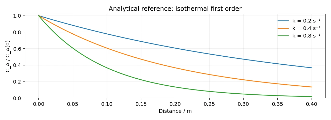
Deep dive · Package script: first_order_reference.py, and the reactor with axial dispersion
#!/usr/bin/env python3
# SPDX-License-Identifier: GPL-3.0-or-later
"""Analytical first-order *isothermal* reference, NOT OpenFOAM flame kinetics."""
import argparse
import csv
from math import exp
from pathlib import Path


def main():
    p = argparse.ArgumentParser(description=__doc__)
    p.add_argument("--k", type=float, default=0.4, help="Reaction constant in 1/s")
    p.add_argument("--u", type=float, default=0.08, help="Constant plug-flow speed in m/s")
    p.add_argument("--length", type=float, default=0.4, help="Reactor length in m")
    p.add_argument("--output", type=Path, default=Path("reference_first_order.csv"))
    a = p.parse_args()
    if a.k < 0 or a.u <= 0 or a.length <= 0:
        p.error("Need k>=0, u>0, length>0")
    if a.output.exists():
        p.error("Output already exists; no overwrite")
    with a.output.open("x", newline="", encoding="utf-8") as handle:
        w = csv.writer(handle)
        w.writerow(["x_m", "t_s", "C_over_C0", "conversion_X"])
        for i in range(101):
            x = a.length * i / 100
            t = x / a.u
            frac = exp(-a.k*t)
            w.writerow([f"{x:.8g}", f"{t:.8g}", f"{frac:.12g}", f"{1-frac:.12g}"])
    print(f"Wrote analytical reference: {a.output}; Da = {a.k*a.length/a.u:.6g}")


if __name__ == "__main__":
    main()
Test with the guide values (k = 0.4 s⁻¹, u = 0.08 m/s, L = 0.4 m): Da = kL/u = 2 and outlet conversion 1 − e⁻² = 0.8647, as in the last CSV row; the second command shows the overwrite protection:
$ python3 ../g18/scripts/first_order_reference.py --k 0.4 --u 0.08 --length 0.4 --output reference_first_order.csv
Wrote analytical reference: reference_first_order.csv; Da = 2
[exit 0]
$ head -4 reference_first_order.csv; tail -2 reference_first_order.csv
x_m,t_s,C_over_C0,conversion_X
0,0,1,0
0.004,0.05,0.980198673307,0.0198013266932
0.008,0.1,0.960789439152,0.0392105608477
0.396,4.95,0.138069237311,0.861930762689
0.4,5,0.135335283237,0.864664716763
[exit 0]
$ python3 ../g18/scripts/first_order_reference.py --output reference_first_order.csv
usage: first_order_reference.py [-h] [--k K] [--u U] [--length LENGTH]
                                [--output OUTPUT]
first_order_reference.py: error: Output already exists; no overwrite
[exit 2]
The plug-flow solution assumes infinite Pe. With axial dispersion and the boundary conditions of P. V. Danckwerts, “Continuous flow systems: distribution of residence times”, Chemical Engineering Science 2, 1–13, 1953, doi:10.1016/0009-2509(53)80001-1 (derived in general form by J. F. Wehner, R. H. Wilhelm, “Boundary conditions of flow reactor”, Chemical Engineering Science 6, 89–93, 1956, doi:10.1016/0009-2509(56)80014-6), the first-order conversion is:
a = sqrt(1 + 4*Da/Pe)
X = 1 - 4*a*exp(Pe/2) / ( (1 + a)^2 * exp(a*Pe/2) - (1 - a)^2 * exp(-a*Pe/2) )| Pe | 10 | 100 | 1000 | ∞ (plug flow) | 0 (perfectly mixed) |
|---|---|---|---|---|---|
| X (Da = 2) | 0.8227 | 0.8594 | 0.8641 | 0.8647 | 0.6667 |
The analytical reference is a verification tool: an isothermal CFD case with uniform velocity and a linear source (for instance a passive species with a sink term) must reproduce these values as the mesh is refined. The methane/air case is not comparable, as the guide stresses.
Deep dive · Damköhler and Péclet numbers of the tutorial flame
- Damköhler: with third-order kinetics there is no k in s⁻¹; the chemical time is defined locally, τ = [CH₄]/ω, and depends on T and composition.
reaction_thermo.pyevaluates it at the stoichiometric composition: 2.6·10⁻⁸ s at 2000 K, 1.1·10⁻⁵ s at 1000 K. With the global strain a = 10 s⁻¹, Da = 1/(a·τ) is 4·10⁶ at 2000 K and 9·10³ at 1000 K. - Domain Péclet: Pe = uL/D = 0.1 × 0.02/2.2·10⁻⁵ ≈ 90 in the cold gas, about 4 at 2000 K: in the hot zone convection and diffusion are comparable, which is why the flame is thick (section 2).
- In diffusion flames strain is better measured by the scalar dissipation rate χ = 2D|∇Z|² at the stoichiometric surface, the variable of flamelet models: N. Peters, “Laminar diffusion flamelet models in non-premixed turbulent combustion”, Progress in Energy and Combustion Science 10, 319–339, 1984, doi:10.1016/0360-1285(84)90114-X. It can be obtained from the Z profile of
paraview_profile.pyand the D of the section 2 table.
13. Quantitative comparisons with physical meaning
Compare A/B/C at the same physical time and on the same plane: peak temperature, reaction-zone location, CH4 and CO2 profiles, volume integral of Qdot when available and species fluxes across the boundaries. When interpreting changes in kinetics, remember that changing A also changes temperature, density and transport.
A maximum concentration or temperature is not a global mass balance. Differences between CFD cases may reflect numerical diffusion, time-step sensitivity or resolution of the mixing layer; distinguish these sources from actual kinetic effects.
Deep dive · Package script: inspect_profiles.py and the synthetic example profiles
#!/usr/bin/env python3
# SPDX-License-Identifier: GPL-3.0-or-later
"""Summarize user-exported ParaView species profiles (not reaction conversion)."""
import argparse
import csv
import math
from pathlib import Path
import sys

REQUIRED = ("x_m", "CH4", "O2", "CO2", "H2O", "T_K")


def summarize(path: Path) -> dict:
    with path.open(newline="", encoding="utf-8-sig") as handle:
        reader = csv.DictReader(handle)
        if not reader.fieldnames or not set(REQUIRED).issubset(reader.fieldnames):
            raise ValueError(f"Required columns: {', '.join(REQUIRED)}")
        rows = []
        for index, rec in enumerate(reader, start=2):
            try:
                values = {k: float(rec[k]) for k in REQUIRED}
            except (ValueError, TypeError):
                raise ValueError(f"Invalid numeric value at row {index}") from None
            if not all(math.isfinite(v) for v in values.values()):
                raise ValueError(f"NaN/Infinity at row {index}")
            for s in ("CH4", "O2", "CO2", "H2O"):
                if values[s] < -1e-6 or values[s] > 1 + 1e-6:
                    raise ValueError(f"Unphysical mass fraction {s} at row {index}")
            rows.append(values)
    if len(rows) < 2:
        raise ValueError("At least two profile points required")
    peak = max(rows, key=lambda r: r["T_K"])
    return {"source": path.name, "points": len(rows), "T_peak_K": peak["T_K"],
            "x_at_T_peak_m": peak["x_m"], "CH4_min": min(v["CH4"] for v in rows),
            "CH4_max": max(v["CH4"] for v in rows),
            "CO2_max": max(v["CO2"] for v in rows)}


def main():
    p = argparse.ArgumentParser(description=__doc__)
    p.add_argument("profiles", nargs="+", type=Path)
    p.add_argument("--output", type=Path, default=Path("summary_profiles.csv"))
    args = p.parse_args()
    if args.output.exists():
        p.error(f"Output exists and will not be overwritten: {args.output}")
    try:
        summaries = [summarize(path) for path in args.profiles]
        with args.output.open("x", newline="", encoding="utf-8") as handle:
            writer = csv.DictWriter(handle, fieldnames=list(summaries[0]))
            writer.writeheader()
            writer.writerows(summaries)
        print(f"Wrote {args.output}; no species conversion inferred from a line profile")
    except (ValueError, OSError) as err:
        print(f"ERROR: {err}", file=sys.stderr)
        sys.exit(2)


if __name__ == "__main__":
    main()
The script requires the six columns x_m,CH4,O2,CO2,H2O,T_K (other columns are allowed and ignored, so it directly accepts the output of paraview_profile.py), rejects non-numeric values, NaN and mass fractions outside [0, 1] and does not overwrite the summary file. Test on the three package examples:
$ python3 ../g18/scripts/inspect_profiles.py A_reference_SYNTHETIC_profile.csv B_half_A_SYNTHETIC_profile.csv C_double_A_SYNTHETIC_profile.csv --output summary_guide18.csv
Wrote summary_guide18.csv; no species conversion inferred from a line profile
[exit 0]
$ cat summary_guide18.csv
source,points,T_peak_K,x_at_T_peak_m,CH4_min,CH4_max,CO2_max
A_reference_SYNTHETIC_profile.csv,41,1238.709,0.019,0.04229478,0.1098828,0.045
B_half_A_SYNTHETIC_profile.csv,41,914.3405,0.019,0.04230124,0.1099414,0.0225
C_double_A_SYNTHETIC_profile.csv,41,1496.444,0.019,0.03113846,0.1097657,0.09
[exit 0]
The three example files, in full. They are synthetic, meant only to test the script, and not representative of the case: the abscissae run from 0 to 0.04 m while the tutorial domain is 0.02 m long; at x = 0 they have YCH4 = 0.11 while the tutorial inlet imposes pure methane; the peak temperatures (914–1496 K) and their differences between B, A and C are very different from what is expected for a flame close to the fast-chemistry limit (section 7). They must not be used as expected values.
examples/A_reference_SYNTHETIC_profile.csv
x_m,CH4,O2,CO2,H2O,T_K
0,0.1098828,0,0.0001597792,0.0002307922,296.3579
0.001,0.108102,0.005493734,0.0002848372,0.0004114315,298.9861
0.002,0.1062656,0.01097835,0.0004921545,0.0007108899,303.343
0.003,0.1043466,0.0164456,0.0008242037,0.001190517,310.3213
0.004,0.1023101,0.02188227,0.001337815,0.001932399,321.1152
0.005,0.1001138,0.02726849,0.002104678,0.00304009,337.2314
0.006,0.09770994,0.03257638,0.003209251,0.004635584,360.4448
0.007,0.09505024,0.03776958,0.004742965,0.00685095,392.677
0.008,0.09209248,0.04280426,0.006793984,0.009813532,435.7807
0.009,0.08880982,0.04763236,0.009432512,0.01362474,491.2313
0.01,0.08520086,0.05220758,0.01269283,0.01833409,559.7494
0.011,0.08129906,0.05649379,0.01655457,0.02391216,640.9068
0.012,0.07717907,0.06047529,0.02092694,0.03022781,732.7954
0.013,0.07295773,0.0641669,0.02564023,0.03703588,831.8486
0.014,0.06878808,0.06762185,0.03044852,0.0439812,932.8985
0.015,0.06484583,0.07093481,0.03504604,0.05062205,1029.519
0.016,0.06130963,0.07423797,0.03909668,0.05647298,1114.646
0.017,0.058338,0.07768968,0.04227359,0.06106185,1181.411
0.018,0.05604686,0.08145627,0.04430234,0.06399227,1224.047
0.019,0.05449231,0.08569,0.045,0.065,1238.709
0.02,0.05366189,0.09050697,0.04430234,0.06399227,1224.047
0.021,0.0534765,0.0959696,0.04227359,0.06106185,1181.411
0.022,0.05380233,0.1020772,0.03909668,0.05647298,1114.646
0.023,0.05447049,0.1087667,0.03504604,0.05062205,1029.519
0.024,0.05530022,0.1159232,0.03044852,0.0439812,932.8985
0.025,0.05612133,0.1233979,0.02564023,0.03703588,831.8486
0.026,0.05679214,0.1310298,0.02092694,0.03022781,732.7954
0.027,0.05721045,0.1386666,0.01655457,0.02391216,640.9068
0.028,0.05731694,0.1461812,0.01269283,0.01833409,559.7494
0.029,0.05709203,0.1534821,0.009432512,0.01362474,491.2313
0.03,0.05654802,0.160516,0.006793984,0.009813532,435.7807
0.031,0.05571911,0.1672653,0.004742965,0.00685095,392.677
0.032,0.05465133,0.1737407,0.003209251,0.004635584,360.4448
0.033,0.053394,0.179972,0.002104678,0.00304009,337.2314
0.034,0.05199365,0.1859993,0.001337815,0.001932399,321.1152
0.035,0.05049027,0.1918654,0.0008242037,0.001190517,310.3213
0.036,0.0489159,0.1976102,0.0004921545,0.0007108899,303.343
0.037,0.04729464,0.2032681,0.0002848372,0.0004114315,298.9861
0.038,0.04564364,0.2088664,0.0001597792,0.0002307922,296.3579
0.039,0.04397452,0.2144255,8.687044e-05,0.0001254795,294.8256
0.04,0.04229478,0.2199597,4.57775e-05,6.612306e-05,293.962
examples/B_half_A_SYNTHETIC_profile.csv
x_m,CH4,O2,CO2,H2O,T_K
0,0.1099414,0,7.988959e-05,0.0001153961,295.2062
0.001,0.1082049,0.005496867,0.0001424186,0.0002057158,296.9329
0.002,0.1064405,0.01098917,0.0002460773,0.0003554449,299.7955
0.003,0.1046348,0.0164728,0.0004121019,0.0005952583,304.3802
0.004,0.1027704,0.02194114,0.0006689074,0.0009661995,311.472
0.005,0.1008261,0.02738424,0.001052339,0.001520045,322.0605
0.006,0.09877805,0.03278819,0.001604625,0.002317792,337.3119
0.007,0.09660205,0.03813479,0.002371483,0.003425475,358.4888
0.008,0.09427701,0.04340213,0.003396992,0.004906766,386.8084
0.009,0.09178952,0.04856618,0.004716256,0.00681237,423.24
0.01,0.08913889,0.05360379,0.006346416,0.009167046,468.2571
0.011,0.08634184,0.0584969,0.008277287,0.01195608,521.5784
0.012,0.08343569,0.06323764,0.01046347,0.0151139,581.9502
0.013,0.08047887,0.06783345,0.01282011,0.01851794,647.0291
0.014,0.07754789,0.07231093,0.01522426,0.0219906,713.42
0.015,0.07473061,0.0767174,0.01752302,0.02531103,776.9005
0.016,0.07211635,0.08111898,0.01954834,0.02823649,832.83
0.017,0.06978438,0.08559484,0.02113679,0.03053092,876.6954
0.018,0.06779266,0.09022814,0.02215117,0.03199613,904.7075
0.019,0.06616923,0.095095,0.0225,0.0325,914.3405
0.02,0.06490787,0.1002535,0.02215117,0.03199613,904.7075
0.021,0.06396902,0.1057348,0.02113679,0.03053092,876.6954
0.022,0.06328578,0.1115386,0.01954834,0.02823649,832.83
0.023,0.06277371,0.1176334,0.01752302,0.02531103,776.9005
0.024,0.06234242,0.1239616,0.01522426,0.0219906,713.42
0.025,0.06190682,0.1304489,0.01282011,0.01851794,647.0291
0.026,0.06139607,0.1370149,0.01046347,0.0151139,581.9502
0.027,0.06075907,0.1435833,0.008277287,0.01195608,521.5784
0.028,0.05996616,0.1500906,0.006346416,0.009167046,468.2571
0.029,0.05900755,0.156491,0.004716256,0.00681237,423.24
0.03,0.05788939,0.162758,0.003396992,0.004906766,386.8084
0.031,0.05662879,0.1688826,0.002371483,0.003425475,358.4888
0.032,0.05524874,0.1748703,0.001604625,0.002317792,337.3119
0.033,0.05377392,0.180736,0.001052339,0.001520045,322.0605
0.034,0.05222759,0.1864997,0.0006689074,0.0009661995,311.472
0.035,0.05062975,0.1921827,0.0004121019,0.0005952583,304.3802
0.036,0.04899641,0.1978051,0.0002460773,0.0003554449,299.7955
0.037,0.04733963,0.2033841,0.0001424186,0.0002057158,296.9329
0.038,0.04566797,0.2089332,7.988959e-05,0.0001153961,295.2062
0.039,0.04398726,0.2144627,4.343522e-05,6.273976e-05,294.1995
0.04,0.04230124,0.2199799,2.288875e-05,3.306153e-05,293.6321
examples/C_double_A_SYNTHETIC_profile.csv
x_m,CH4,O2,CO2,H2O,T_K
0,0.1097657,0,0.0003195584,0.0004615843,297.273
0.001,0.1078964,0.005487467,0.0005696744,0.000822863,300.6175
0.002,0.1059158,0.01095669,0.0009843091,0.00142178,306.1618
0.003,0.10377,0.01639121,0.001648407,0.002381033,315.0419
0.004,0.1013894,0.02176454,0.002675629,0.003864798,328.7775
0.005,0.09868905,0.02703697,0.004209356,0.006080181,349.2858
0.006,0.09557374,0.03215276,0.006418501,0.009271169,378.8257
0.007,0.09194664,0.03703917,0.00948593,0.0137019,419.8421
0.008,0.08772343,0.04160852,0.01358797,0.01962706,474.6929
0.009,0.0828504,0.04576473,0.01886502,0.02724948,545.2556
0.01,0.07732479,0.04941515,0.02538567,0.03666818,632.4471
0.011,0.0712135,0.05248759,0.03310915,0.04782433,735.7224
0.012,0.06466583,0.05495057,0.04185389,0.06045561,852.6536
0.013,0.05791547,0.05683379,0.05128045,0.07407177,978.7019
0.014,0.05126847,0.05824371,0.06089705,0.0879624,1107.291
0.015,0.04507627,0.05936962,0.07009207,0.1012441,1230.243
0.016,0.03969619,0.06047594,0.07819336,0.112946,1338.571
0.017,0.03544522,0.06187936,0.08454718,0.1221237,1423.531
0.018,0.03255526,0.06391255,0.08860468,0.1279845,1477.787
0.019,0.03113846,0.06688,0.09,0.13,1496.444
0.02,0.03116993,0.07101394,0.08860468,0.1279845,1477.787
0.021,0.03249145,0.0764392,0.08454718,0.1221237,1423.531
0.022,0.03483543,0.08315442,0.07819336,0.112946,1338.571
0.023,0.03786407,0.09103341,0.07009207,0.1012441,1230.243
0.024,0.04121583,0.09984636,0.06089705,0.0879624,1107.291
0.025,0.04455036,0.1092958,0.05128045,0.07407177,978.7019
0.026,0.04758429,0.1190596,0.04185389,0.06045561,852.6536
0.027,0.05011321,0.1288332,0.03310915,0.04782433,735.7224
0.028,0.0520185,0.1383624,0.02538567,0.03666818,632.4471
0.029,0.05326097,0.1474641,0.01886502,0.02724948,545.2556
0.03,0.05386526,0.1560319,0.01358797,0.01962706,474.6929
0.031,0.05389976,0.1640306,0.00948593,0.0137019,419.8421
0.032,0.0534565,0.1714814,0.006418501,0.009271169,378.8257
0.033,0.05263416,0.178444,0.004209356,0.006080181,349.2858
0.034,0.05152575,0.1849986,0.002675629,0.003864798,328.7775
0.035,0.05021131,0.1912307,0.001648407,0.002381033,315.0419
0.036,0.04875488,0.1972204,0.0009843091,0.00142178,306.1618
0.037,0.04720466,0.2030363,0.0005696744,0.000822863,300.6175
0.038,0.04559497,0.2087328,0.0003195584,0.0004615843,297.273
0.039,0.04394904,0.2143509,0.0001737409,0.000250959,295.3232
0.04,0.04228187,0.2199194,9.155501e-05,0.0001322461,294.2242
Practical tip · An A/B/C comparison table with the source of every number
| Quantity | Tool | Expected (sections 1 and 7) |
|---|---|---|
| O₂ and CH₄ conversion (steady window) | species_balance.py | O₂ close to 100 %; CH₄ ≤ 10.4 % |
| ∫Qdot dV and −Σhfw | species_balance.py | equal to each other, ≤ 136.6 W, nearly equal in A, B, C |
| mass and element residuals | species_balance.py | small (≲ 0.1 %) |
| peak T | Tmax / inspect_profiles.py | ≤ 2305 K, small differences |
| position of peak T and of Zst on the axis | paraview_profile.py | close to each other, on the air side, almost unchanged |
| Qdot peak and width | paraview_profile.py | peak increasing and width decreasing from B to A to C |
| number of steps and run time | log.foamRun | time increasing with A (stiffer chemistry) |
Always report the time, the line and the averaging window used; values are for the 20 mm thickness of the mesh.
14. Numerical verification and uncertainty
Repeat at least the reference case with a refined mesh and stricter time stepping (or a smaller maxCo), reporting changes in the observables. Verify inlet conditions, kinetic-mechanism units, elemental conservation and ODE integration behavior. Scientific conclusions also require appropriate experimental validation; the tutorial’s global mechanism is not valid for all methane combustion conditions.
Optional refresher — Chemical convergence. Chemical timescales may be much faster than flow timescales. A fluid-dynamically stable run can still underresolve the reaction layer. Courant number alone is not a complete measure of kinetic integration error.
Practical tip · The numerical variants, with the commands
Each variant in a new copy of the reference case, prepared before the run (as in the section 7 box, updating GUIDE18_VARIANT.txt) and with the monitors installed:
cd "$HOME/cfd_guide18_cases"
# 1) mesh twice as fine in x and y (0.1 x 0.25 mm)
sed -i 's/(100 40 1)/(200 80 1)/' M_fine/system/blockMeshDict
# 2) smaller Courant number
foamDictionary -entry maxCo -set 0.2 T_co02/system/controlDict
# 3) tighter ODE tolerance (tutorial: relTol 1e-1)
sed -i 's/^\(\s*relTol\s\+\)1e-1;/\11e-3;/' O_tol/constant/chemistryProperties
grep -n "hex\|maxCo\|relTol" M_fine/system/blockMeshDict T_co02/system/controlDict O_tol/constant/chemistryProperties- For each variant compare the quantities of the section 13 table with A. With three meshes (factor 2) the observed order and the GCI convergence index can be estimated: P. J. Roache, “Perspective: a method for uniform reporting of grid refinement studies”, Journal of Fluids Engineering 116, 405–413, 1994, doi:10.1115/1.2910291; I. B. Celik et al., “Procedure for estimation and reporting of uncertainty due to discretization in CFD applications”, Journal of Fluids Engineering 130, 078001, 2008, doi:10.1115/1.2960953 (Guide 4).
- The quantity most sensitive to the mesh is the Qdot peak, because the reaction zone is thinner than the mixing layer; integral heat release and conversion are much less sensitive.
- The ODE tolerance variant is the cheapest and often the most instructive:
relTol 1e-1accepts 10 % relative errors in the chemistry integration of each step. - Refinement must not change the physical problem: same boundary conditions and same thickness in z. To start from an already burning solution
mapFieldscan be used (section 5).
Deep dive · Stiff chemistry: how OpenFOAM 14 integrates the reactions within the step
- At every step, for every cell, the
Standardchemistry model integrates the ODE system of concentrations and temperature at constant pressure over the interval Δt, with its own sub-steps; the result gives the mean ratesRRused in the species equations and in Qdot. It is a splitting between transport and chemistry: the splitting error grows with Δt. seulexis a variable-order linearly implicit Euler extrapolation method, suitable for stiff systems (E. Hairer, G. Wanner, Solving Ordinary Differential Equations II: Stiff and Differential-Algebraic Problems, Springer, 1996, doi:10.1007/978-3-642-05221-7).absTolandrelTolcontrol the local error;initialChemicalTimeStep 1e-07is the first sub-step, then adapted. With τchem of 10⁻⁸ s in the hot zone (section 3) the system is stiff and an explicit method would need thousands of sub-steps.- The
Courant numbercontrols transport accuracy, not chemistry accuracy: this is why the guide warns that it is not enough. The section 14 variants (ODE tolerance,maxCo, mesh) separate the three contributions.
15. Extending the approach to a liquid chemical reactor
For an isothermal liquid reactor, define the species balances, liquid diffusivities, measured reaction kinetics (possibly concentration- and pH-dependent), geometry, flow regime and boundary conditions. Do not reuse the tutorial’s perfectGas thermodynamics or methane combustion law. Heterogeneous reactions require an appropriate surface model and boundary conditions; liquid-liquid extraction requires the phases and interfacial mass transfer to be modelled first.
This case therefore teaches the reasoning behind transport plus reactive source terms. It is not a universal chemistry simulator without further model development, calibration and verification.
Deep dive · Towards a liquid-phase reactor in OpenFOAM 14: what changes in the files
- Thermodynamics: instead of
hePsiThermo/perfectGasuseheRhoThermowith a liquid equation of state available in OpenFOAM 14 (rhoConst,rPolynomial,perfectFluid,icoPolynomial,rhoTabulated),hConstoreConstthermodynamics andconstorAndradetransport (liquid viscosity as a function of T). - Diffusion:
FickianFourierwith measured diffusivities (section 2), typically 10⁻⁹ m²/s: the Schmidt number is about 1000, a thousand times that of a gas. - Kinetics: measured laws, with orders and units consistent with concentrations in kmol/m³ (
CH4^0.2syntax for non-stoichiometric orders, units in square brackets as inreverseBurner, section 3). Equilibrium reactions in solution are written as forward/backward pairs or with the reversible types. - Reaction engineering references: O. Levenspiel, Chemical Reaction Engineering, 3rd ed., Wiley, 1999; H. S. Fogler, Elements of Chemical Reaction Engineering, Prentice Hall; for residence time distribution, Danckwerts (1953, section 12).
Practical tip · In a liquid numerical diffusion exceeds physical diffusion: check it before trusting the conversion
A first-order scheme introduces a numerical diffusivity of order u·Δx/2. With u = 0.08 m/s and 1 mm cells it is 4·10⁻⁵ m²/s, forty thousand times the molecular diffusivity of a solute (10⁻⁹ m²/s); even a bounded second-order scheme stays far above the physical value near strong gradients. In a mixing-controlled reaction the computed conversion then measures the mesh, not the chemistry. Countermeasures: very fine meshes in the mixing zones, less diffusive schemes, a check against the analytical reference of section 12 and, in stirred reactors, turbulence and mixing models suited to high Schmidt numbers.
16. Final checklist
- ☐ OpenFOAM Foundation 14 version checked.
- ☐ Case folders are isolated copies; original tutorials untouched.
- ☐ Changes to Arrhenius
Adocumented and no other changes made. - ☐
checkMesh, logs andfoamRunoutput reviewed. - ☐ No obviously unphysical mass fractions, temperature or heat release.
- ☐ Profiles compared at matching times, planes and color scales.
- ☐ Conversion and balances based on fluxes, not an isolated mass fraction.
- ☐ Numerical sensitivity and mechanism limitations stated.
Practical tip · The checklist with the command or script that verifies it
| Item | How to verify it |
|---|---|
| Foundation 14 version | foamVersion → OpenFOAM-14; echo $WM_PROJECT_VERSION |
| isolated copies, original intact | diff "$FOAM_TUTORIALS/multicomponentFluid/counterFlowFlame2D/constant/reactions" A_reference/constant/reactions (only the format of A) |
| only A changed | diff -r A_reference B_half_A (only reactions and GUIDE18_VARIANT.txt; log.* and results aside) |
| mesh and run checked | grep -E "Mesh OK|Failed" log.checkMesh, tail -n 2 log.foamRun → End |
| physical fields | cellMin/cellMax (section 9), T ≤ 2305 K, Y ≥ 0 |
| comparison at same time and line | paraview_profile.py, inspect_profiles.py (section 10) |
| conversion from fluxes | species_balance.py with the monitors of add_monitors.py |
| numerical sensitivity and mechanism limits | section 14 variants; comparison with reaction_thermo.py and the T(Z) curve |
References and license
- OpenFOAM Foundation 14 —
counterFlowFlame2Dtutorial - OpenFOAM Foundation 14 —
constant/reactions - OpenFOAM 14 — release notes and chemistry updates
Original educational material and scripts: GNU GPL v3 or later; original OpenFOAM files retain their own license and attribution. Illustrative data are not CFD results; no experimentally validated outputs are claimed.
Deep dive · Annotated bibliography and OpenFOAM 14 sources consulted
Combustion and diffusion flames
- C. K. Law, Combustion Physics, Cambridge University Press, 2006, doi:10.1017/CBO9780511754517.
- F. A. Williams, Combustion Theory, 2nd ed., CRC Press (reissue 2018), doi:10.1201/9780429494055.
- N. Peters, Turbulent Combustion, Cambridge University Press, 2000, doi:10.1017/CBO9780511612701.
- T. Poinsot, D. Veynante, Theoretical and Numerical Combustion, 3rd ed., 2012.
- S. P. Burke, T. E. W. Schumann, “Diffusion flames”, Ind. Eng. Chem. 20, 998–1004, 1928, doi:10.1021/ie50226a005.
- A. Liñán, Acta Astronautica 1, 1007–1039, 1974, doi:10.1016/0094-5765(74)90066-6.
- Y. Tsuji, Prog. Energy Combust. Sci. 8, 93–119, 1982, doi:10.1016/0360-1285(82)90015-6.
- N. Peters, Prog. Energy Combust. Sci. 10, 319–339, 1984, doi:10.1016/0360-1285(84)90114-X.
- K. Seshadri, N. Peters, Combust. Flame 73, 23–44, 1988, doi:10.1016/0010-2180(88)90051-X.
- M. D. Smooke, I. K. Puri, K. Seshadri, Symp. (Int.) Combust. 21, 1783–1792, 1988, doi:10.1016/S0082-0784(88)80412-0.
Mechanisms and mixture fraction
- C. K. Westbrook, F. L. Dryer, Combust. Sci. Technol. 27, 31–43, 1981, doi:10.1080/00102208108946970.
- W. P. Jones, R. P. Lindstedt, Combust. Flame 73, 233–249, 1988, doi:10.1016/0010-2180(88)90021-1.
- R. W. Bilger, S. H. Stårner, R. J. Kee, Combust. Flame 80, 135–149, 1990, doi:10.1016/0010-2180(90)90122-8.
- GRI-Mech 3.0.
- M. N. Bui-Pham, PhD thesis, University of California, San Diego, 1992 (source of the tutorial mechanism).
Thermophysical properties and transport
- C. R. Wilke, J. Chem. Phys. 18, 517–519, 1950, doi:10.1063/1.1747673.
- W. Sutherland, Phil. Mag. 36, 507–531, 1893, doi:10.1080/14786449308620508.
- B. J. McBride, M. J. Zehe, S. Gordon, NASA/TP-2002-211556, 2002.
- J. O. Hirschfelder, C. F. Curtiss, R. B. Bird, Molecular Theory of Gases and Liquids, Wiley, 1954.
- V. Giovangigli, Multicomponent Flow Modeling, Birkhäuser, 1999, doi:10.1007/978-1-4612-1580-6.
- R. J. Kee, M. E. Coltrin, P. Glarborg, Chemically Reacting Flow, Wiley, 2003, doi:10.1002/0471461296.
Numerical methods and verification
- E. Hairer, G. Wanner, Solving Ordinary Differential Equations II, Springer, 1996, doi:10.1007/978-3-642-05221-7.
- S. B. Pope, Combust. Theory Model. 1, 41–63, 1997, doi:10.1080/713665229.
- F. Contino et al., Proc. Combust. Inst. 33, 3057–3064, 2011, doi:10.1016/j.proci.2010.08.002.
- P. J. Roache, J. Fluids Eng. 116, 405–413, 1994, doi:10.1115/1.2910291.
- I. B. Celik et al., J. Fluids Eng. 130, 078001, 2008, doi:10.1115/1.2960953.
Reaction engineering
- P. V. Danckwerts, Chem. Eng. Sci. 2, 1–13, 1953, doi:10.1016/0009-2509(53)80001-1.
- J. F. Wehner, R. H. Wilhelm, Chem. Eng. Sci. 6, 89–93, 1956, doi:10.1016/0009-2509(56)80014-6.
- O. Levenspiel, Chemical Reaction Engineering, 3rd ed., Wiley, 1999.
OpenFOAM 14 sources cited in the boxes
- applications/modules/multicomponentFluid/thermophysicalPredictor.C
- src/thermophysicalModels/chemistryModel/Standard/Standard_chemistryModel.C
- src/thermophysicalModels/specie/reaction/reactionRate/ArrheniusReactionRate/ArrheniusReactionRateI.H
- src/ThermophysicalTransportModels/fluid/laminar/unityLewisFourier/unityLewisFourier.H
- src/ThermophysicalTransportModels/fluid/laminar/FickianFourier/FickianFourier.H
- src/thermophysicalModels/specie/transport/sutherland/sutherlandTransportI.H
- src/functionObjects/field/specieFlux/specieFlux.H
- src/functionObjects/field/fieldValues/volFieldValue/volFieldValue.C
- etc/caseDicts/functions/combustion/Qdot
- tutorials/multicomponentFluid/membrane/system/functions
- tutorials/multiRegion/CHT/reverseBurner/constant/gas/reactions
- applications/utilities/mesh/manipulation/checkMesh/checkMesh.C
Related guides: Linux server from Windows, monitoring and convergence, ParaView for quantitative analysis, verification and validation, parameter sweeps, mesh generation and quality checks, boundary conditions and physical models, transient simulations, turbulence and RANS models, heat transfer and natural convection, conjugate heat transfer, species transport, diffusion and mixing, multiphase flows and VOF interfaces, porous media and pressure loss, rotating machinery, MRF and fans, dynamic meshes and moving walls, dispersed particles and wall interaction and the Learning OpenFOAM 14 path.
Download: scripts and files of the guide
The archive OpenFOAM14_Guida18_script.zip (42 kB compressed, 14 files) contains every script and data file reproduced or cited in this article, with the same content as the boxes: the scripts/, examples/ and similar folders hold the guide package files, extra/ the additional scripts and files presented in the deep dives. README_IT_EN.txt lists the contents with SHA-256 checksums; files marked SYNTHETIC are illustrative data, not CFD results. Licence GNU GPL v3 or later (COPYING_GPLv3.txt).
Recommended order: python3 scripts/prepare_cases.py "$HOME/cfd_guide18_cases", then, before the run, python3 extra/add_monitors.py on every copy (species fluxes per patch, masses, integrated Qdot at every step, section 9) and finally bash scripts/run_case.sh. Numbers to expect before the run: python3 extra/reaction_thermo.py <case> (sections 1 and 3); species, element and energy balances: python3 extra/species_balance.py <case> (section 11); profiles exported from ParaView: python3 extra/paraview_profile.py (section 10).
Archive contents:
examples/A_reference_SYNTHETIC_profile.csv— SYNTHETIC / illustrative data, not CFD results (42 lines)examples/B_half_A_SYNTHETIC_profile.csv— SYNTHETIC / illustrative data, not CFD results (42 lines)examples/C_double_A_SYNTHETIC_profile.csv— SYNTHETIC / illustrative data, not CFD results (42 lines)extra/add_monitors.py— Install the Guide 18 balance monitors in a NEW counterFlowFlame2D copy.extra/functions_guide18— system/functions for counterFlowFlame2D written by add_monitors.py: Qdot every step, specie fluxes per patch, specie masses, heat release, reactionRates, Tmaxextra/make_synthetic_monitors.py— SYNTHETIC test data for species_balance.py – NOT OpenFOAM results.extra/make_synthetic_paraview.py— SYNTHETIC ParaView-style 'Plot Over Line' CSV to test paraview_profile.py.extra/paraview_profile.py— converts a ParaView Plot Over Line CSV to x_m,CH4,O2,CO2,H2O,T_K (+ N2, Qdot, Bilger mixture fraction) and locates T peak, Z_st and the Qdot peakextra/reaction_thermo.py— A-priori thermochemistry of the counterFlowFlame2D case (OpenFOAM 14).extra/species_balance.py— Species, element and energy balances of a counterFlowFlame2D run (OpenFOAM 14).scripts/first_order_reference.py— Analytical first-order *isothermal* reference, NOT OpenFOAM flame kinetics.scripts/inspect_profiles.py— Summarize user-exported ParaView species profiles (not reaction conversion).scripts/prepare_cases.py— Prepare isolated Arrhenius-sensitivity cases from OpenFOAM Foundation 14.scripts/run_case.sh— Run one newly prepared OpenFOAM 14 case; never clean or overwrite old output.