

Four-Point Calibration with Linear Axes
In this chapter (V07) a four-point scientific calibration is built and verified.
1. A Linear Scientific Graph as the Source
To make the test reproducible, a fully synthetic PNG was created, 1280 × 900 pixels, with a slightly perspective quadrilateral scientific grid and two colored traces. The figure is not an experimental observation and does not represent already published numerical data.
The horizontal axis is Elapsed time, from 0 to 10 s; the vertical axis is Signal, from −20 to 80 mV. Four small targets identify the physical corners of the scientific rectangle; a fifth, yellow target marks a known control point, 5 s, 30 mV.
The image was imported as a canonical image.raster Dataset into an independent Session, using the public Acquisition Handler, and then associated with a Digitizer Configuration through the actual Preview source image → Use this image dialog.
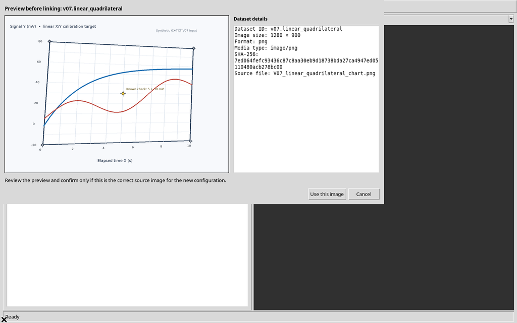
The initial window shows the image and its metadata. The visible traces still belong to the raster pixels: in V07 they are not digitized or published as scientific curves.
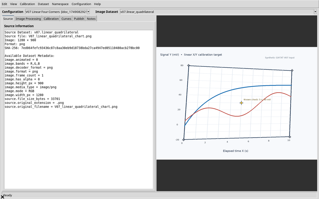
2. The Calibration Tab and Its Functions
Select the Calibration tab on the left side of the Viewer. At the top, X axis and Y axis are shown, each with Label, Unit, Semantic role, Minimum, Maximum and Scale, followed by Apply axis settings.
Further down are the A · Full image and B · Scale bar options. These belong to other calibration modes; they are not the four-point procedure of this chapter.
The Projective calibration and verification panel, instead, contains the Set BL, Set BR, Set TL, Set TR and Clear corners buttons, the geometric status of the calibration and the Verify calibration… command.
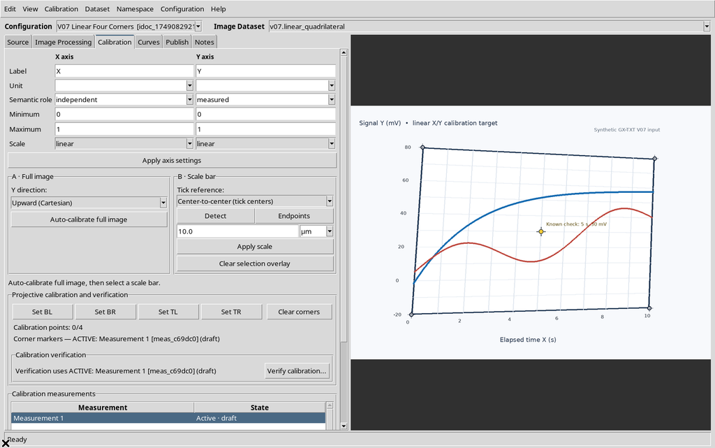
The order BL/BR/TL/TR stands respectively for bottom-left, bottom-right, top-left and top-right of the physical graph. They must not be confused with the corners of the whole image when the graph occupies only part of it.
3. The Calibration Must Be Complete Before Verification
A new Digitizer Configuration does not contain the four scientific corners. If you press Verify calibration… before completing the calibration and defining valid axes, the GUI shows:
Complete the four-corner calibration and valid scientific axes before verifying a known point.
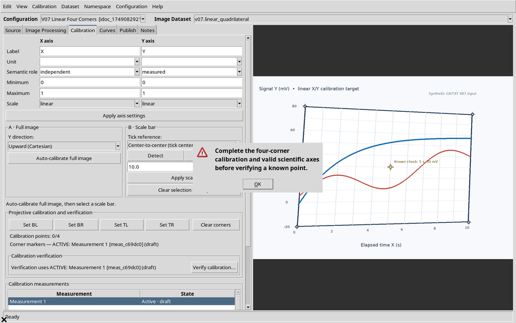
The rejection was observed directly; it did not create a fictitious calibration or modify the Dataset. It is a useful safeguard that prevents verifying coordinates that do not yet have an established physical meaning.
4. Setting Linear X/Y Axes and Validating the Limits
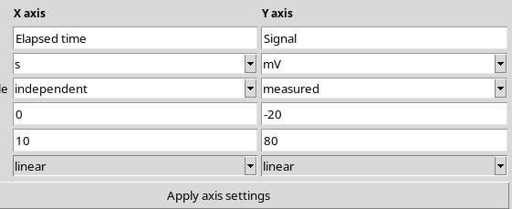
Enter Elapsed time in the Label field of the X axis, s as Unit, Minimum 0, Maximum 10 and Scale linear. For Y enter Signal, mV, Minimum −20, Maximum 80, Scale linear. The Semantic role entries are independent and measured respectively.
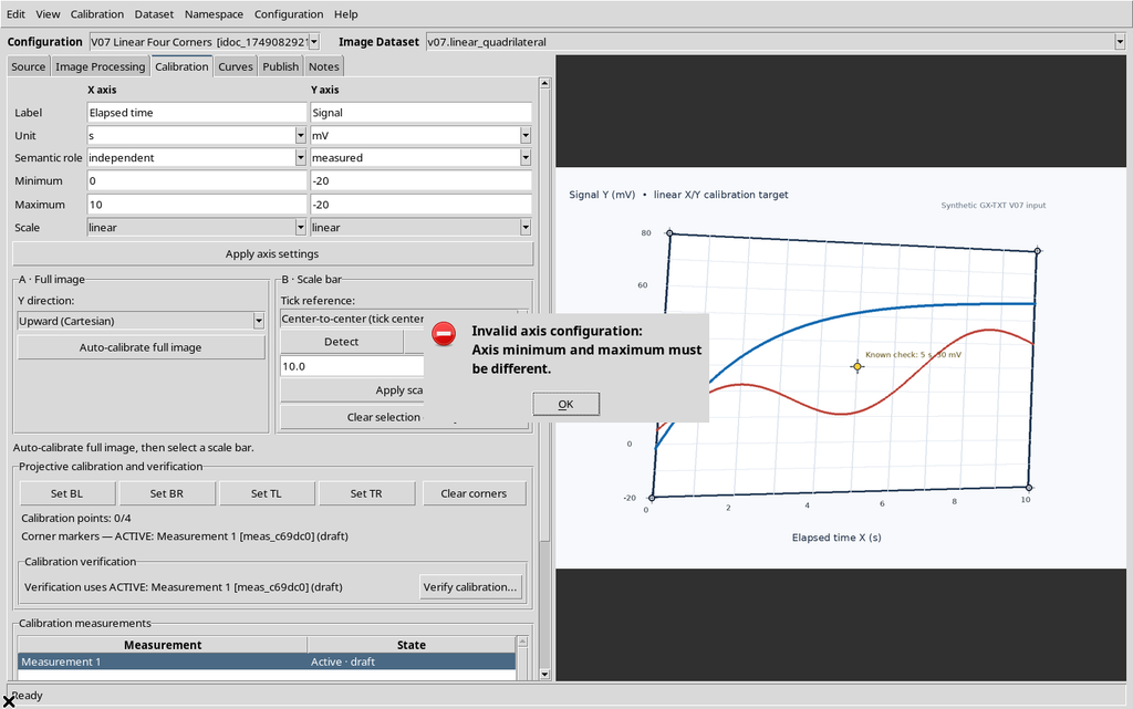
Before accepting the correct configuration, a negative test was run: setting both Y Minimum and Maximum to −20, Apply axis settings showed Axis minimum and maximum must be different.
Once the upper Y limit was restored to 80, Apply axis settings saved both linear definitions in the Workspace. The four corners were still missing: the axis limits and the geometric calibration are distinct objects.
This chapter considers only Scale = linear for both axes. Logarithmic or mixed axes, with positivity conditions and different transformations, will be the subject of guide V08.
5. The Four Clicks: BL, BR, TL and TR
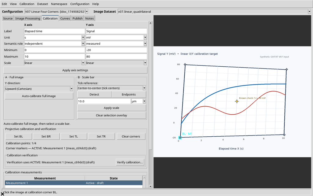
The procedure is guided one button at a time. Press Set BL, then click the target at the bottom left of the graph area. Repeat with Set BR at the bottom right, Set TL at the top left and finally Set TR at the top right.
The Viewer shows the light-blue/cyan markers and a counter Calibration points: 1/4, then 2/4, 3/4, until completion.
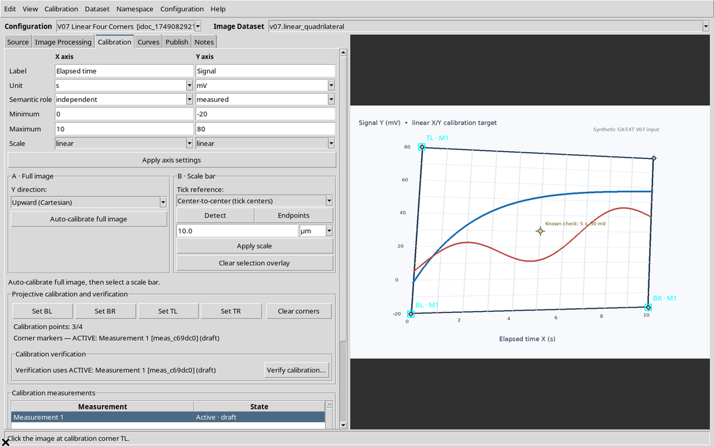
The authoritative state stored the coordinates in source pixels, which are not necessarily integers even when the pointer produces events on integer window pixels: the inverse viewport transformation keeps the resulting values.
6. A Controlled Error: Four Degenerate Points
To document a recoverable error, the fourth point, TR, was initially placed deliberately at the same position as TL. Formally there were four entries in the document, but not four geometrically independent corners.
The viewer showed Calibration invalid: Degenerate calibration points.
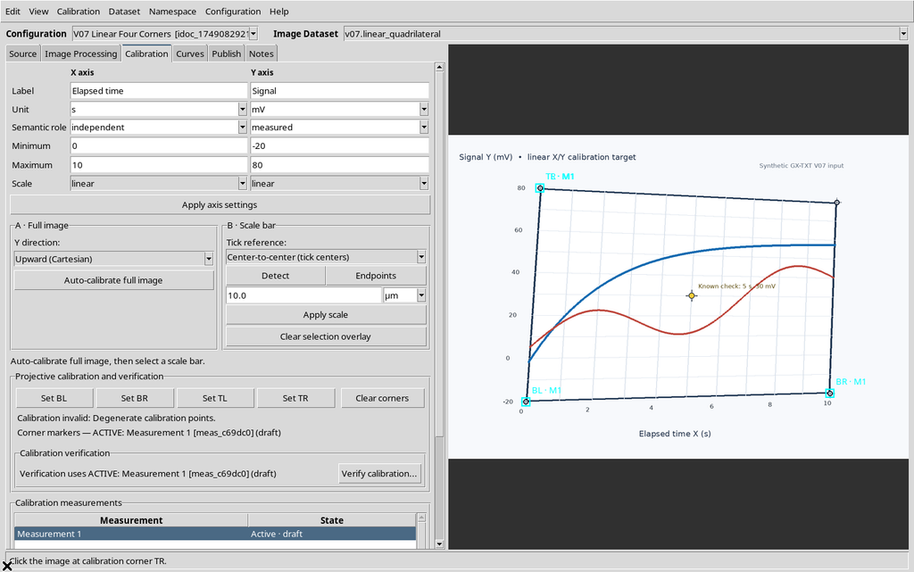

This result shows that 4/4 stored points is not always the same as a valid calibration. The numerical check of the matrix recognizes the degeneracy.
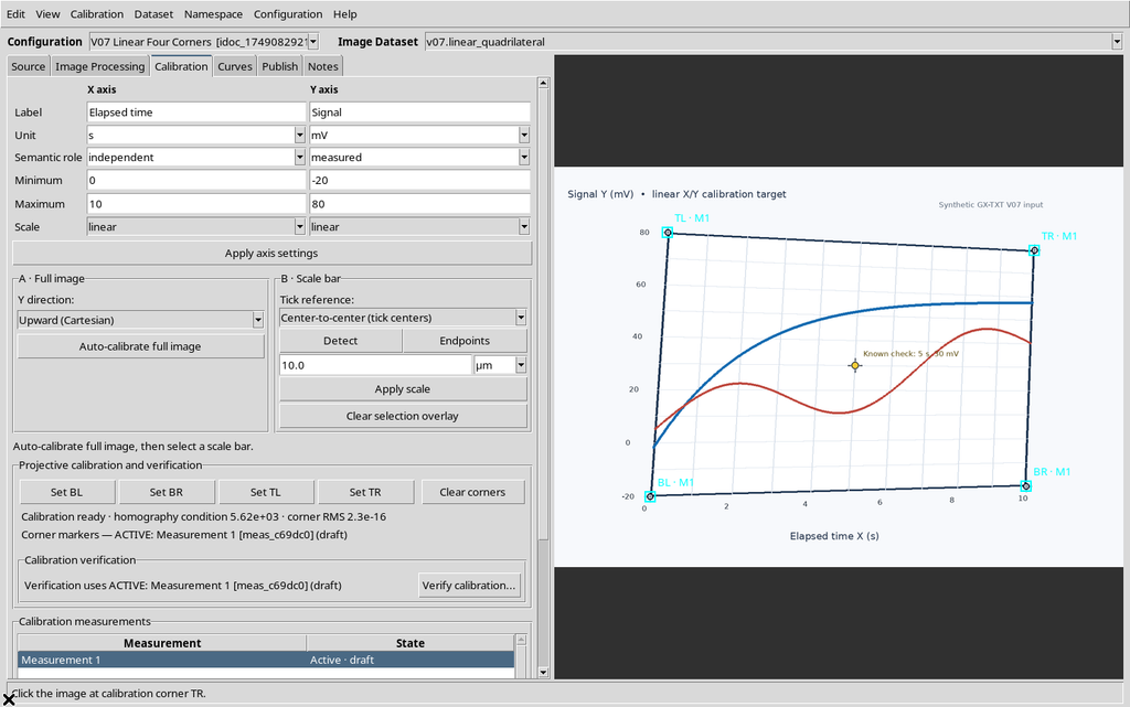
Repeating Set TR and clicking the correct target at the top right, the status became Calibration ready and the four markers outlined the original quadrilateral.
7. How the Projective Transformation Is Built
The GX-TXT model determines a homography from four pairs of coordinates. The corners of the raster are associated with normalized coordinates:
| Corner | Normalized X | Normalized Y |
|---|---|---|
| BL | 0 | 0 |
| BR | 1 | 0 |
| TL | 0 | 1 |
| TR | 1 | 1 |
A 3×3 matrix transforms the original pixels (p_x,p_y) into normalized coordinates (u,v), dividing by the third homogeneous component. The linear scientific axes are applied afterwards:
X = Xmin + u × (Xmax − Xmin)
Y = Ymin + v × (Ymax − Ymin)
This distinguishes two concepts: linear numerical axes and perspective geometry of the figure. A tilted chart or printout may require a projective transformation even when the X/Y quantities are linear.

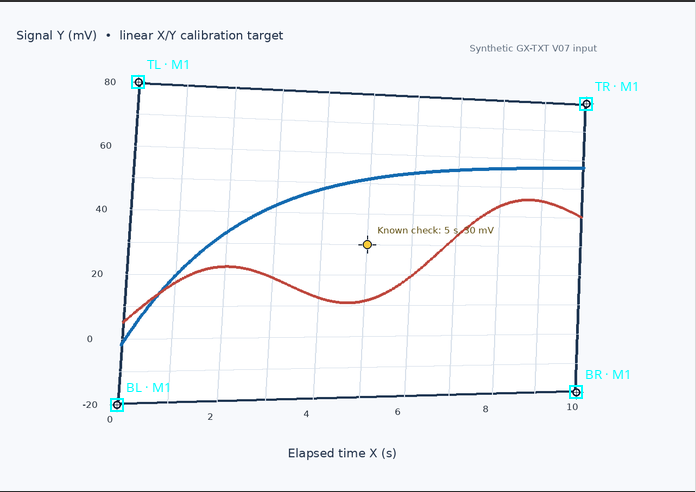
The quadrilateral of the fixture is not a perfect parallelogram. The CORE matrix has non-zero projective terms; it was not arbitrarily replaced with an affine transformation.
8. Matrix Condition and Corner RMS
In the run, the tab shows Calibration ready · homography condition 5.62e+03 · corner RMS 2.3e−16.
These numbers describe the geometric solution computed from the four points actually clicked:
- homography condition: numerical indicator of the conditioning of the matrix used;
- corner RMS: reprojection error of the four corners in normalized coordinates.
An almost-zero RMS is expected when a homography passes exactly through the four points used to determine it. It does not prove the experimental precision of the graph reading, nor does it quantify the uncertainty in mouse positioning or in the production of the image.
To check whether the calibration correctly represents other positions, you must use known points independent of the corners. This is done in the next step.
9. Opening the Integrated Scientific Verification
With four valid corners, press Verify calibration…. The Viewer expands a Calibration verification section directly in the same tab, without opening a separate verification application.
The two blocks show the actual names and units X · Elapsed time [s, linear] and Y · Signal [mV, linear]; each contains Expected, Calculated, Δ physical and Relative / log.
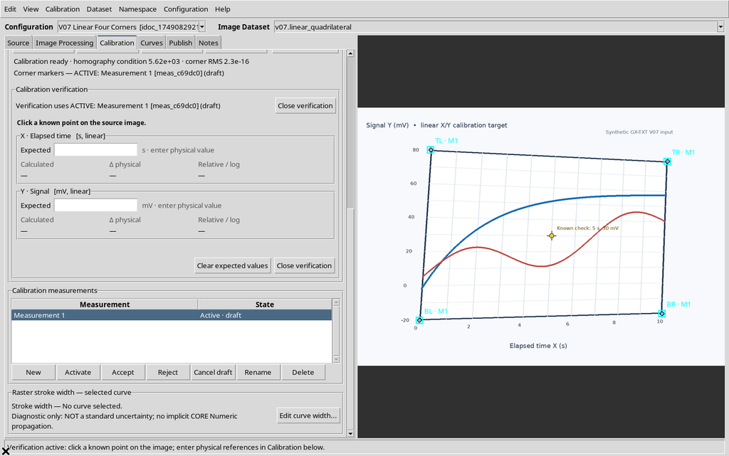
In the test this procedure uses the calibration of the active Measurement 1, which is still in the draft state. The geometric calibration can be valid without the realization having been formally accepted in the measurement manager. The life cycle of groups and measurements is documented in V09.
10. The Known Point: 5 s and 30 mV
The fixture contains a yellow control marker, geometrically placed at 5 s, 30 mV and not used to build the homography.
That marker was clicked on the actual canvas. The viewer resolved the click to the approximate source position (675.9137; 445.3957) px, then showed the calculated values even before the Expected values were entered.
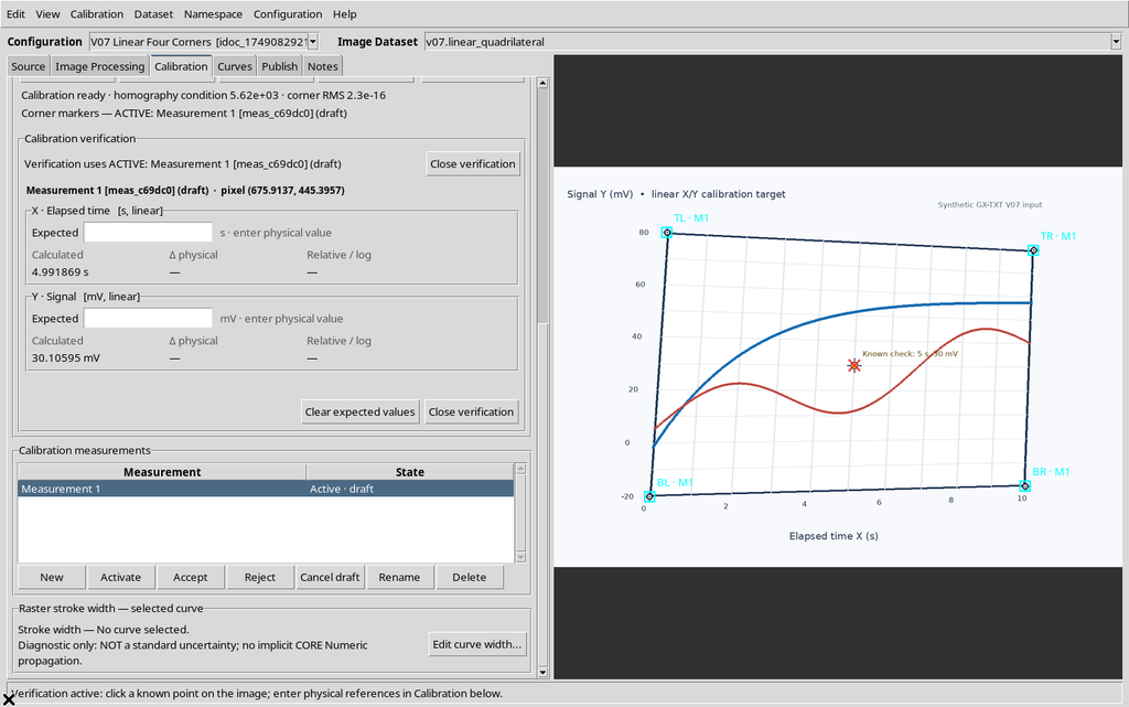
Entering Expected X = 5 s and Expected Y = 30 mV, the interface returned:
| Quantity | Calculated value | Reference | Physical Δ |
|---|---|---|---|
| X · Elapsed time | 4.991869 s | 5 s | −0.008130769 s |
| Y · Signal | 30.10595 mV | 30 mV | +0.1059471 mV |
The displayed relative deviations were about −0.1626154% for X and +0.3531569% for Y.
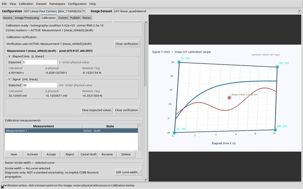
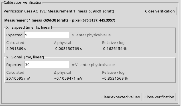
This is the residual of a control point, not a general estimate of the dispersion, the uncertainty or the quality of all future digitized curves.
11. Invalid Expected References and Clearing Them
The Expected field is not confused with the calculated value. Deliberately entering non-numeric text for X, the interface showed Invalid reference, while still displaying the calculated geometric result.
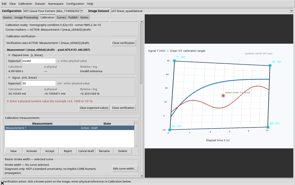
The Clear expected values button emptied the comparison fields, returning the residuals to the no-reference state. It did not delete the four corners or modify the image.
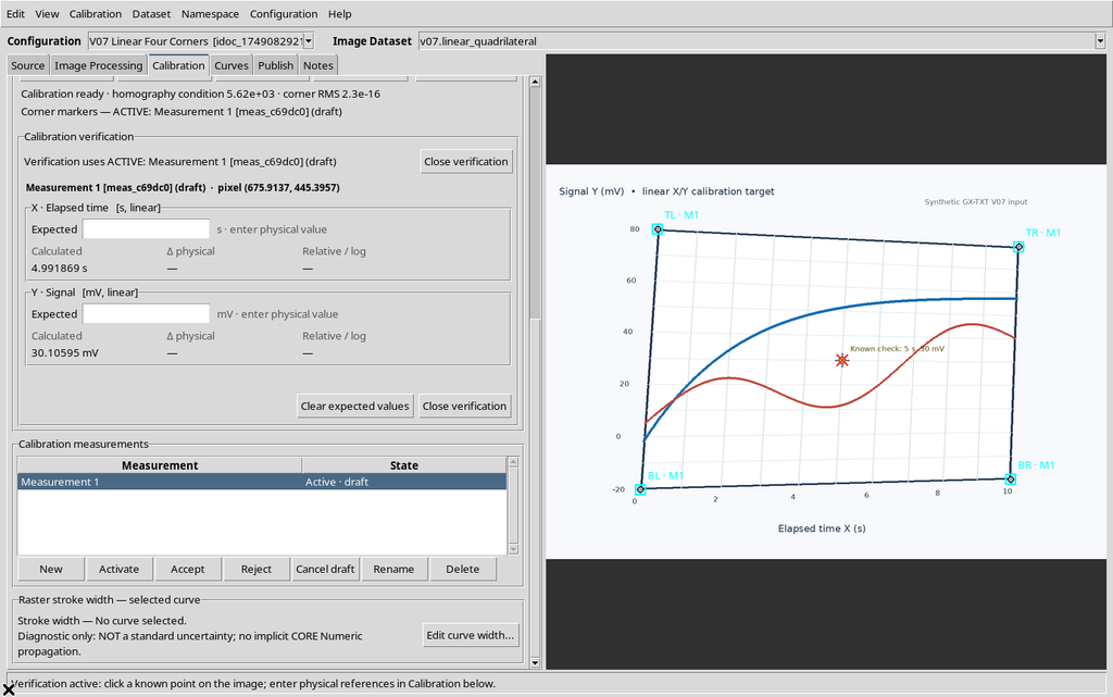
The 5 s and 30 mV references were then entered again: the panel reproduced the same values. Close verification finally closed the panel to continue with the normal calibration operations.
12. Correcting a Corner Already Acquired
To change a specific corner, press its button again, for example Set BL, and click another position on the raster. There is no need to clear the other three markers.
In the example the BL point was temporarily moved, while BR, TL, TR and the X/Y ranges stayed unchanged. The GUI recalculated the matrix and kept the Calibration ready status.
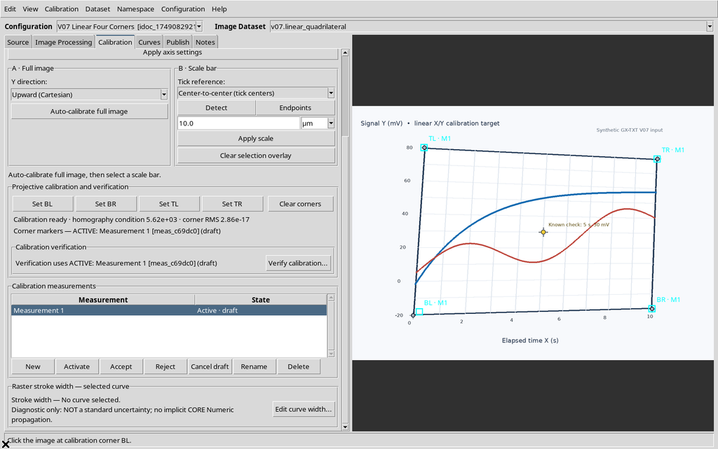
A change of this kind alters the transformation of every pixel and can change the physical values assigned to points of curves already digitized: it is not a simple change of the color or position of the marker.
13. Undo and Redo on Changes to the Four Points
The Edit → Undo menu returned the BL corner exactly to its previous position, and Edit → Redo reapplied the move.
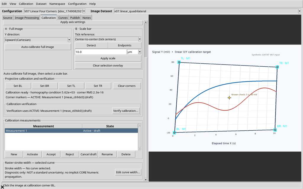
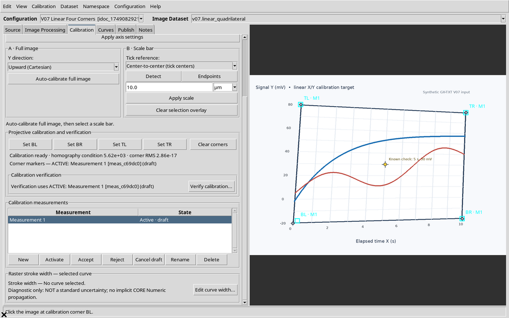
A further Undo restored the initial calibration. The comparison showed that the whole dictionary of the four corners and of the scientific axes was preserved, with the canonical image unchanged.
This verifies the history of a calibration change in the test Session, not Undo/Redo operations on curves and proposals, which will be covered in the dedicated chapters.
14. Clear corners and Restoring
The Clear corners button removes the four geometric points and sets the counter back to Calibration points: 0/4. In the example the linear X/Y axes remain defined, but without corners they do not form a usable transformation.
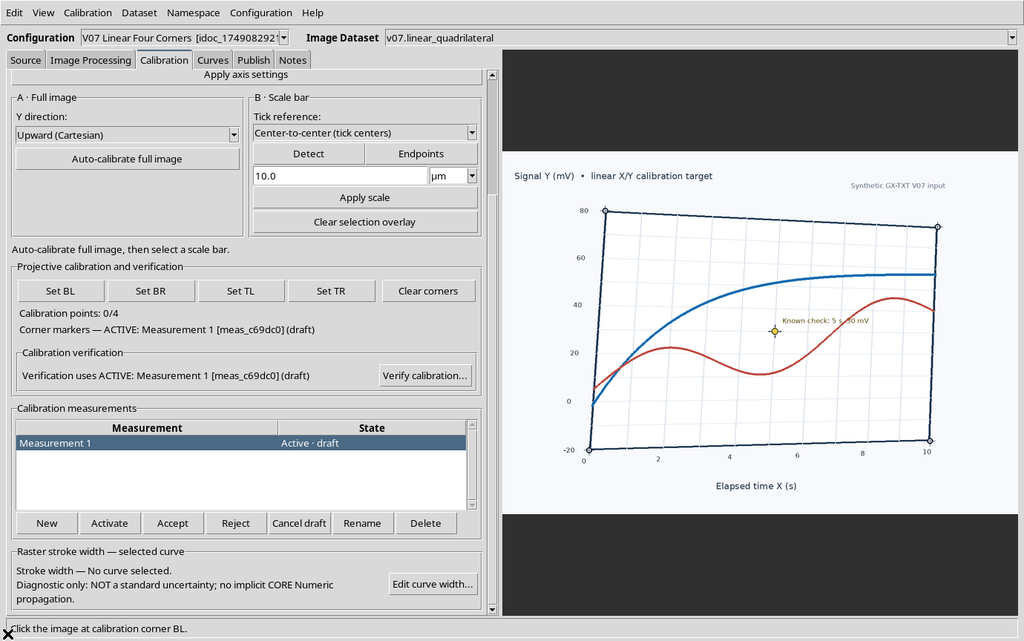
Edit → Undo was used immediately: all four corners and the Calibration ready status were restored.
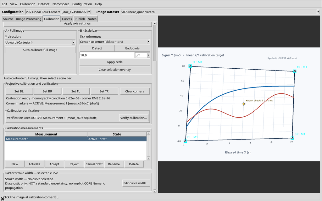
Clear corners must not be confused with Reset physical scale… (V06), nor with deleting the scientific configuration: they are distinct operations with different implications.
15. Changing the Scientific Limits Without Re-clicking the Corners
The axis limits can be changed through Apply axis settings even when the quadrilateral is already defined. X Maximum was temporarily set from 10 to 20 s, leaving X Minimum = 0, Y from −20 to 80 mV and the corners exactly unchanged.
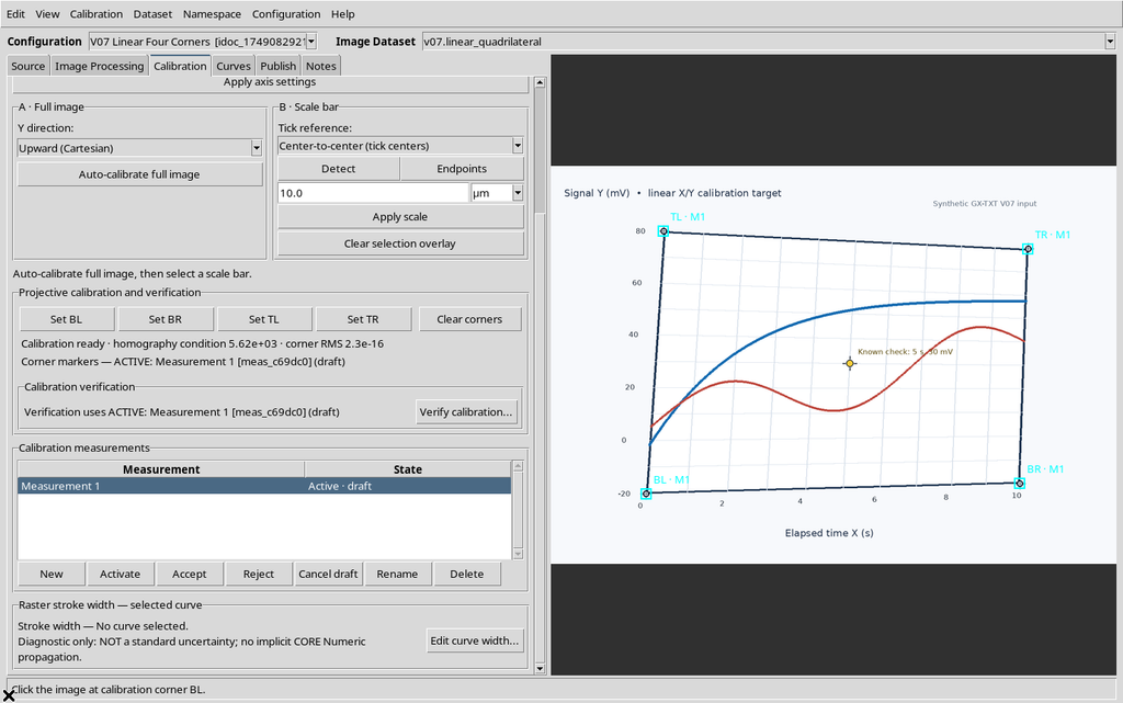
The geometric transformation of the pixels into u,v stays the same, but the linear mapping u→X doubles: the central control point, which previously represented about 5 s, is now interpreted as about 10 s.
The initial configuration X Maximum = 10 was then reapplied, and the CORE confirmed corners, axes and Dataset identical to the reference configuration.
This is a scientific change, not a form of canvas zoom.
16. Visibility of the Calibration Markers
From the View menu you can control Show calibration corners. With a complete calibration, the cyan markers BL · M1, BR · M1, TL · M1 and TR · M1 are actually drawn around the quadrilateral.
Turning the item off, the markers disappear from the image:
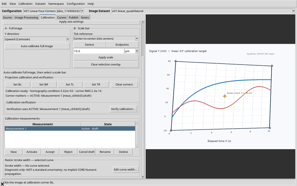
Turning it back on, they return to the same position:
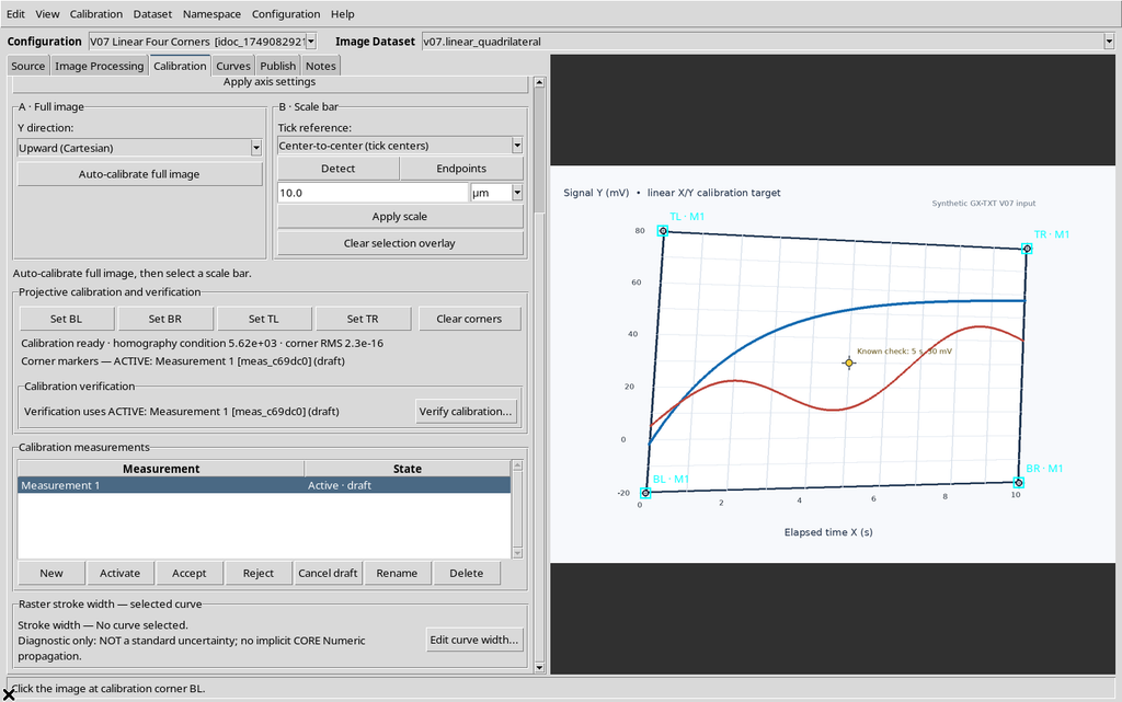
Hiding the markers is a presentation operation; Clear corners is a scientific change.
17. Saving and Reopening in the Same Session
The final configuration, with axes Elapsed time (s) from 0 to 10 and Signal (mV) from −20 to 80, was saved with the actual Configuration → Save configuration command. The Viewer was closed normally and reopened from the framework Digitalizer panel in the same Session.
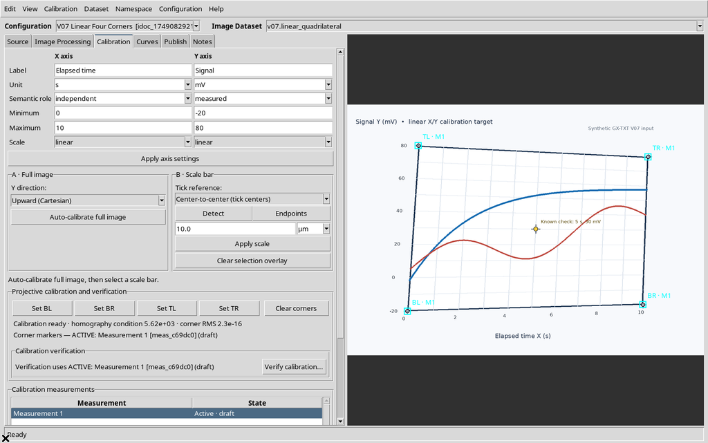
The four points, the axes, the Workspace ID, the canonical source, the measurement group and the Calibration ready status were all found again. The cyan markers were also repainted in the GUI. The image did not change its SHA-256.
This check demonstrates persistence and restoration within the same Session, not a test of recovery after a crash, an external change to the source or a transfer between different Sessions.
18. Scientific Limits and Unverified Conditions
Projective calibration mathematically reconstructs the transformation from the four identified corners. It cannot determine by itself how accurate the printed targets, the reference coordinates or the operator’s pointing are.
The value corner RMS ≈ 0 does not prove zero uncertainty. The measurement on a single independent point is a spot check, not a statistical characterization. With real scientific data it would be advisable to check several points spread over the area, the quality of the raster and the origin of the physical axis limits.
19. Operational Summary
To calibrate a linear graph: import the image as an Image Dataset, create a Digitizer Configuration, fill in Label / Unit / Minimum / Maximum / Scale=linear for both axes and press Apply axis settings. Then select, one at a time, Set BL, Set BR, Set TL and Set TR, clicking the actual corners of the graph area. Check Calibration ready and do not interpret the corner RMS as proof of absolute precision.
Use Verify calibration… on a known physical point independent of the corners, enter the Expected values, read the residuals and assess whether they are compatible with the needs of the experiment. Correct the corners with their respective buttons, use Undo/Redo when appropriate, and save the Workspace.