

Logical Y1/Y2 Axes: Configuration, Verification and Curve Links
This chapter (V10) checks the logical scientific axes Y1 and Y2 of Curve Digitalizer, from enabling them to persistence, including different scales, error dialogs and the links of individual curves. All the commands described were run on the actual GUI.
1. Synthetic Image and Source Dataset
A new isolated Session contains a synthetic scientific PNG of 1280 × 900 pixels, imported through the Acquisition Handler as a canonical image.raster Image Dataset. The figure includes a perspective grid, two colored traces in the raster and four identifiable corners; the annotation distinguishes the blue trace intended for Y1 from the red one intended for Y2.
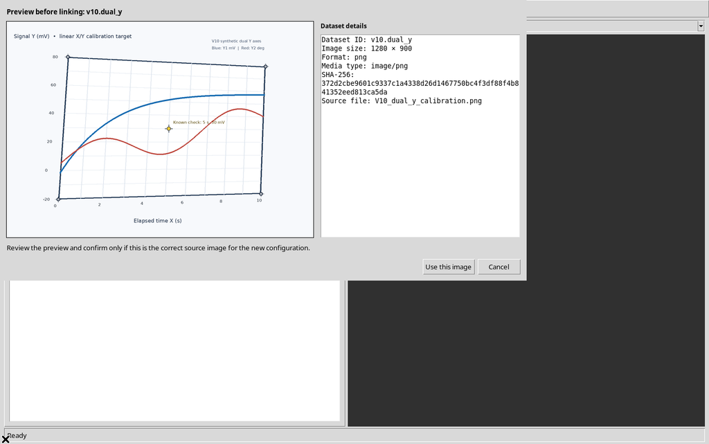
The traces are still original PNG pixels, not digitized numerical curves, and must not be confused with the two placeholder curves that will be created in the GUI.
2. Initial Configuration and Four Corners
At startup the Calibration tab exposes only X axis and Y axis. In this test, X Elapsed time, from 0 to 10 s, and the initial Y Amplitude, from −20 to 80 mV, were applied, both linear.
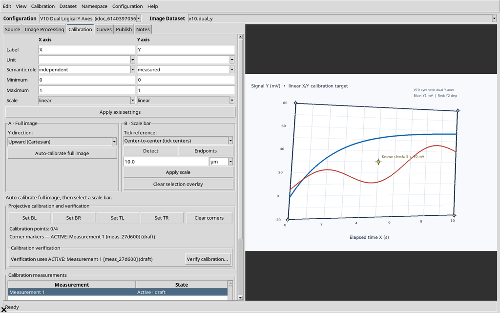
With Set BL, Set BR, Set TL and Set TR, four actual clicks on the raster targets were recorded. The indicator showed Calibration ready and a valid geometric transformation.
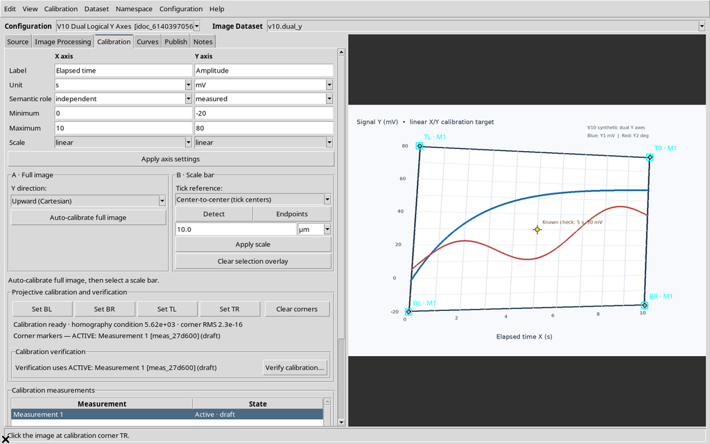
The active realization is still a Measurement 1 (draft): having four valid corners and having formally accepted the measurement are two distinct conditions, already documented in V09.
3. Enabling the Secondary Axis from the Viewer settings Window
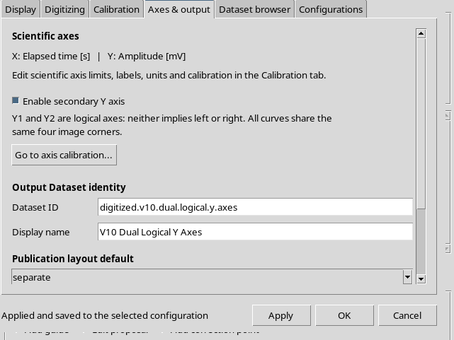
The command is Configuration → Viewer settings… → Axes & output → Enable secondary Y axis.
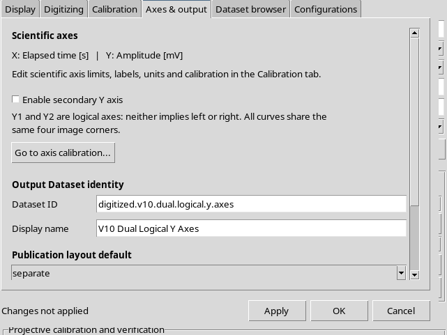
Ticking the checkbox initially changes only the draft in the settings window.
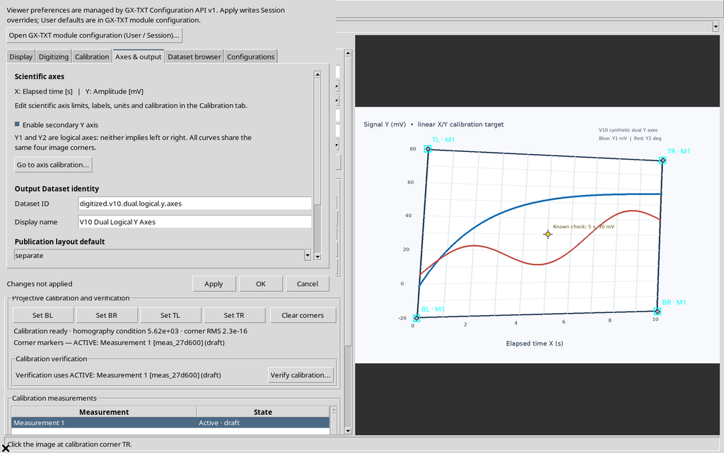
After Apply, the GUI stated Applied and saved to the selected configuration and the secondary axis was added to the scientific document.
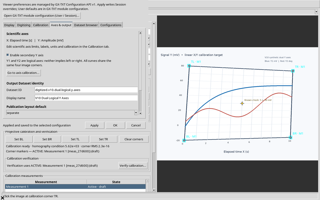
Apply is a non-closing command: the window stays available for examining the configuration.
4. X, Y1 and Y2 in the Same Panel
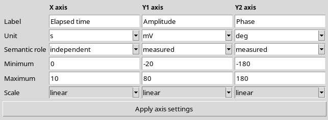
The Calibration tab now shows three columns: X axis, Y1 axis, Y2 axis.
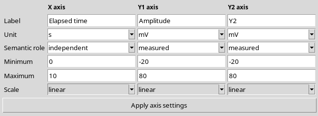
The old Y becomes the logical axis Y1. When first enabled, Y2 inherits the limits, unit and scale of Y1: in this test −20…+80 mV, linear, with the default name Y2. The CORE keeps the same four corners and adds axes.y2 to the model and to the current calibration measurement.
The axes are logical, not a geographic constraint: the software does not automatically assign Y1 to the left side and Y2 to the right. Both use the same pixels and the same homography.
5. Independent Constraints for a Logarithmic Y2
Setting Y2 Scale = log and Minimum = 0, Apply axis settings showed:
Invalid axis configuration: Logarithmic axes require positive limits.
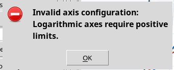
A second attempt with Minimum = −1 was rejected in the same way.
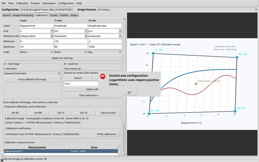
The two invalid drafts changed neither the saved axis definitions nor the calibration corners. This requirement applies to every logarithmic axis; Y1, on the other hand, can include zero or negative values when it is linear.
6. Linear X and Y1 with a Logarithmic Y2
The valid definition tested was:
| Axis | Quantity | Unit | Range | Scale |
|---|---|---|---|---|
| X | Elapsed time | s | 0…10 | linear |
| Y1 | Amplitude | mV | −20…80 | linear |
| Y2 | Amplitude ratio | a.u. | 1…1000 | log |
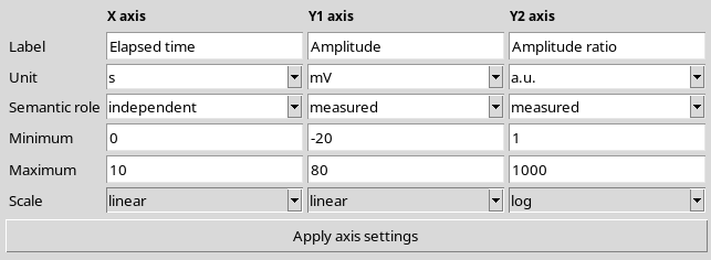
The Viewer saved Y2 as a distinct scientific axis without introducing a second geometric matrix or removing the existing calibration measurement.
7. Simultaneous Verification of X, Y1 and Y2
The Verify calibration… command expands three scientific panels in the same tab. The yellow marker of the raster was clicked on the actual Tk canvas, at event (367,379), corresponding to about (675.9137; 445.3957) source pixels.
With Expected 5 s, 30 mV and √1000 ≈ 31.6227766 a.u., the Viewer displayed:
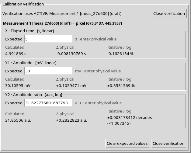
| Axis | Calculated | Δ physical | Relative / log |
|---|---|---|---|
| X | 4.991869 s | −0.008130769 s | −0.1626154 % |
| Y1 | 30.10595 mV | +0.1059471 mV | +0.3531569 % |
| Y2 | 31.85506 a.u. | +0.2322823 a.u. | +0.003178412 decades |
The same original position produces three scientific values according to the assigned axes; the term in decades concerns only the logarithmic Y2.
8. Invalid Y2 Reference and Clearing the Expected Values
With Expected Y2 = 0, the value Calculated Y2 = 31.85506 a.u. stayed visible but the comparison showed Invalid reference, because a logarithmic reference must be strictly positive.
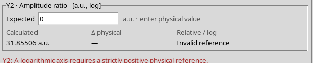
The X and Y1 values stayed correctly calculated. The Clear expected values button then reset the three Expected fields, without changing any scientific calibration.
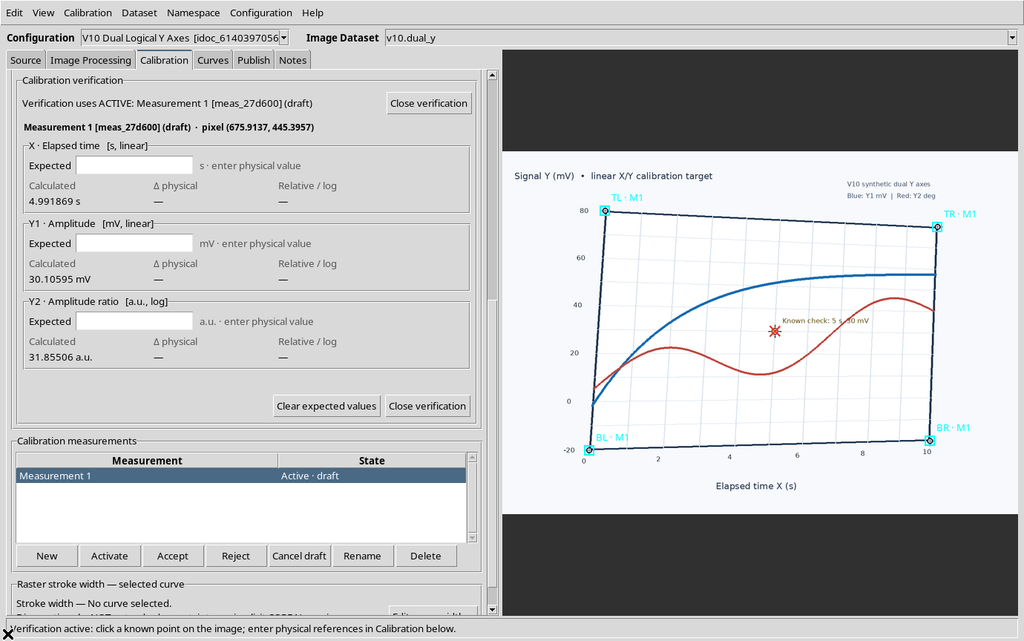
The panel was closed with Close verification. This verification is diagnostic: it does not accept measurements, apply fitting or publish Datasets.
9. A Second Physical Example: Y2 in Degrees
The temporary logarithmic definition was replaced with:
Y1 = Amplitude, −20…80 mV, linear; Y2 = Phase, −180…180 deg, linear.
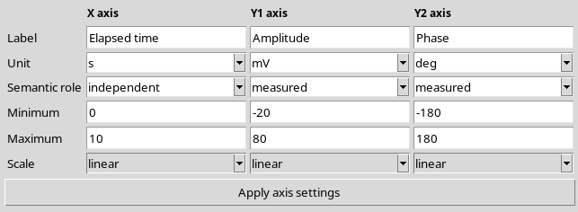
Only the Y2 parameters changed: the name, the unit, the limits and the scale. The X and Y1 axes, the Dataset and the four corners of the raster stayed unchanged.
10. The Same Pixel: 30.10595 mV or 0.3814094°
The verification was repeated on the same source point, with Expected X = 5 s, Y1 = 30 mV and Y2 = 0 deg.
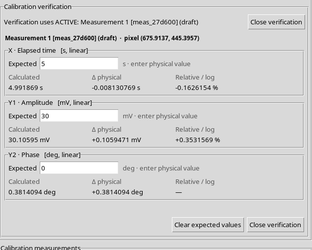
The Viewer showed 4.991869 s, 30.10595 mV and +0.3814094 deg. For Y2 the physical difference is +0.3814094 deg, while the percentage relative to an Expected value of zero is correctly reported as undefined.
The value in degrees is not obtained from the color of the red line; it is the result of the second scientific transformation specified by the operator, applied to the same normalized coordinate.
11. The Curves Tab When Y2 Is Active
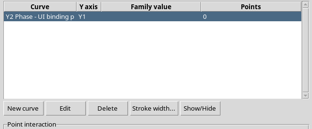
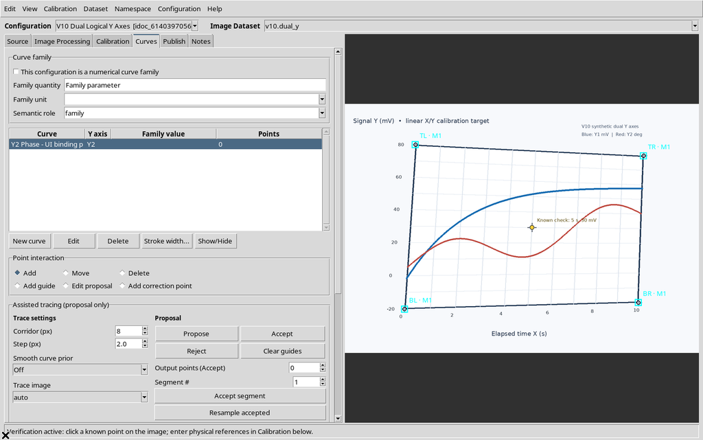
With Y2 enabled, the table in the Curves tab shows an additional Y axis column, besides the curve name, the family value and the number of points.
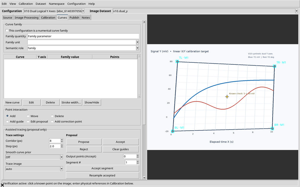
This means that the Y1/Y2 association belongs to the individual curve, not to the perspective calibration of the graph. Enabling Y2 does not by itself assign the colors of the raster to a scientific quantity.
12. The Y axis Selector in New curve
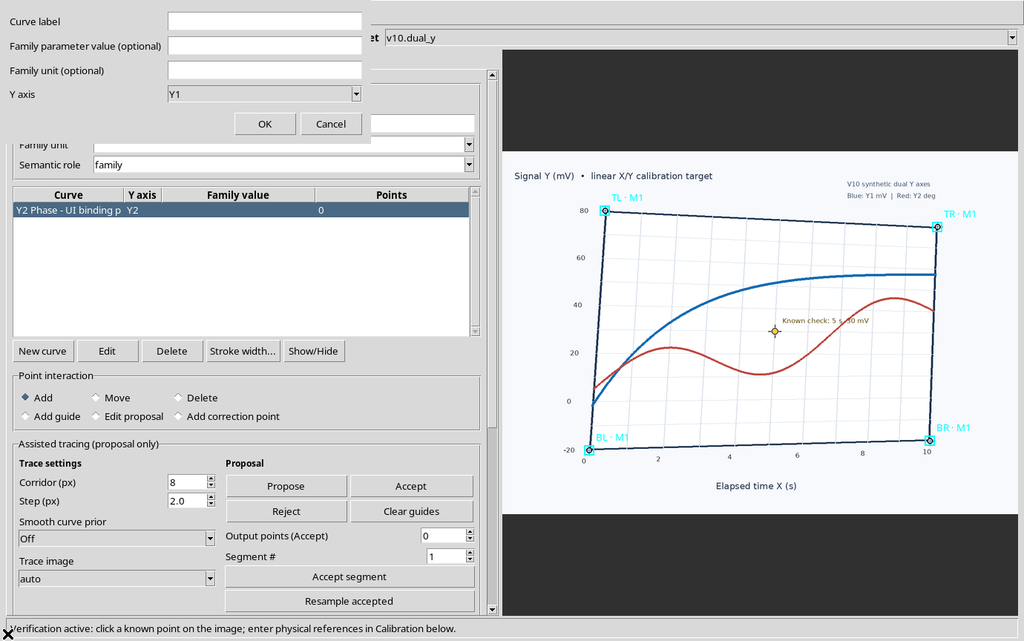
Pressing New curve, the native dialog includes Curve label, an optional family value/unit and Y axis with the Y1 and Y2 options.
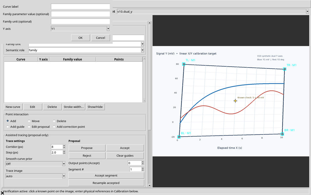
A curve Y2 Phase – UI binding proof was created, assigned to Y2, but with no points.
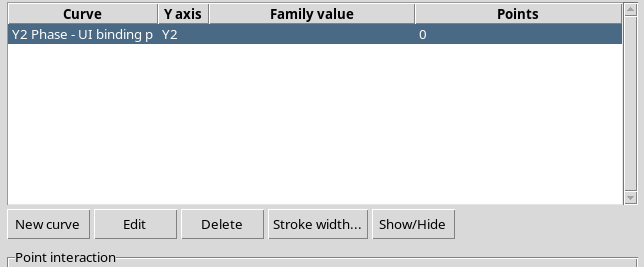
The table showed Y axis = Y2 and Points = 0. This test demonstrates the logical link, not the digitization of the red trace of the source.
13. Protection Against Disabling Y2
With a curve still assigned to Y2, Enable secondary Y axis was unticked. Pressing Apply, the Viewer refused the operation with the warning:
Reassign every Y2 curve to Y1 before disabling Y2.
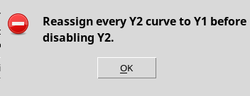
The CORE document stayed unchanged: Y2 axis, curve, ID, four corners and source were not deleted. This is a check built into the software, not a defect.
14. Reassigning the Curve from Y2 to Y1 with Edit
The curve was selected in the Curves tab, then modified with Edit → Y axis = Y1.
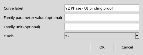
After OK, the same curve was linked to Y1.
Its identifier and the calibration stayed identical.
15. Disabling Y2 After the Reassignment
After reassigning the curve, repeat Enable secondary Y axis → off → Apply. This time the window showed Applied and saved to the selected configuration.
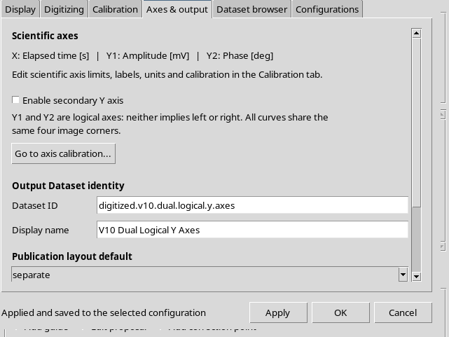
The CORE went back to containing only the x and y axes and also removed y2 from the active measurement, keeping exactly the same four corners.
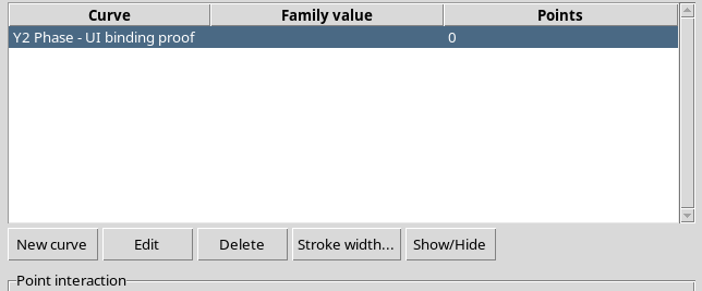
The Curves tab went back to showing the Curve, Family value, Points columns, without Y axis.
16. The Initial Single-Y Model Remains Available
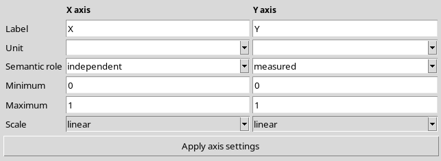
The original structure of the Calibration tab shows only X axis and Y axis, as in the initial configuration.
17. Re-enabling Y2 Recreates the Default Values
Choosing Enable secondary Y axis → on → Apply recreates the Y2 declaration starting from the current Y1.
After this re-enabling the CORE reported Y2, mV, −20…80, linear: the previous Phase definition, which had actually been removed, did not reappear from a hidden preference.
To obtain the desired configuration, Phase, deg, −180…180 had to be set and applied again.
18. Restoring the Y2 Curve and Adding a Y1 Curve
The existing placeholder curve was associated with Y2 again through Edit curve.
New curve was then used to create Y1 Amplitude – UI binding proof, choosing Y1.
The final table showed both associations:
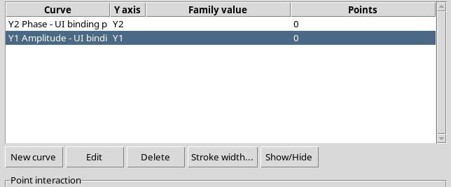
| Placeholder curve | Logical axis | Points |
|---|---|---|
| Y2 Phase – UI binding proof | Y2 | 0 |
| Y1 Amplitude – UI binding proof | Y1 | 0 |
These are two entries in the configuration, not digitized scientific curves, and in particular no published numerical Datasets were produced.
19. A Single Homography, Three Scientific Transformations
The installed model resolves the corners only once and transforms the original pixel into (u,v). In the test:
X = 0 + 10 × u seconds.
Y1 = -20 + 100 × v millivolts.
Y2 = -180 + 360 × v degrees, in the final configuration.
For the temporary logarithmic Y2 configuration: Y2 = 10^(3 × v) arbitrary units.
An independent NumPy calculation, based on the four corners actually recorded and on the same Tk event, obtained X = 4.9918692305 s, Y1 = 30.1059470678 mV, Y2 log = 31.8550588711 a.u. and Y2 Phase = 0.3814094442 deg.
The numerical agreement verifies the software transformation, not the accuracy of a real instrument or the experimental uncertainty.
20. Identity of the Y1/Y2 Model and Canonical Associations
In the Workspace, the two-Y model contains axis_model_version = 2 and the definitions axes.x, axes.y (Y1) and axes.y2 (Y2). Each curve carries its own y_axis_id with the values y1 or y2.
The ID of the Image Dataset and its SHA-256 do not change during enabling, disabling, limit changes or curve reassignment. No other raster and no second homography were created.
The three verification panels X / Y1 / Y2 can use different physical units without implying that the meaning of the Y2 axis is right/left.
21. Save, Close and Reopen in the Same Session
The final configuration was saved with Configuration → Save configuration, then the Viewer was closed and reopened from the normal Viewers → Digitalizer catalog.
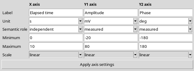
The three axes were restored: X Elapsed time (s), 0…10, Y1 Amplitude (mV), −20…80 and Y2 Phase (deg), −180…180.
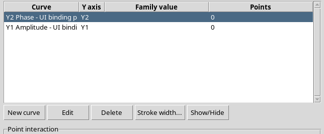
The Curves tab still showed both placeholder curves, assigned to Y2 and Y1 respectively.
The Workspace kept the same document IDs, the calibration group and realization, the four points, the source identity, the axis definitions, the two curve IDs and their respective associations. Neither placeholder had numerical points.
22. Short Practical Procedure
Open the Image Dataset, define the axes and four corners, then choose Configuration → Viewer settings… → Axes & output → Enable secondary Y axis and press Apply.
In the Calibration tab, set Y1 and Y2 with their respective names, units, limits and scientific scales. The limit of a log axis must be positive. Use Apply axis settings, then Verify calibration… on a known point to examine X, Y1 and Y2 at the same time.
In the Curves tab, explicitly assign each series to the corresponding Y axis. Before disabling Y2, move to Y1 all the curves still linked to Y2 through Edit.