

Configuring Image Processing Filters and Their Order
Digitizing a scientific graph can be hindered by insufficient contrast, hard-to-distinguish colors, scanning patterns or noise. The GX-TXT Image Processing tab lets you prepare a sequence of non-geometric filters to apply to the raster. The goal is to improve the readability of the image without changing its geometry, the axis calibration or the points already acquired.
This guide is devoted to the configuration of the filters and to the Standard and Advanced modes. Generating the actual processed preview, comparing the original with the result and publishing a new Image Dataset will be covered separately.
1. Starting from a Known Scientific Source
The example uses a teaching raster of 1280 × 900 pixels containing four colored traces, a grid and slight graininess. The curves represent only synthetic signals, not experimental measurements. The image is already loaded in Curve Digitalizer through an Image Dataset.
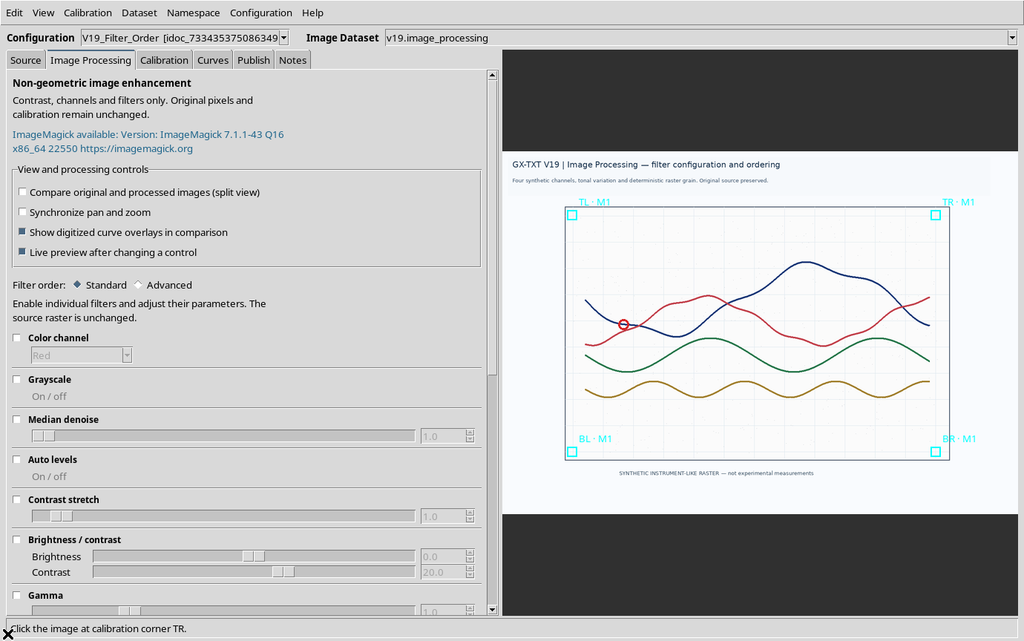
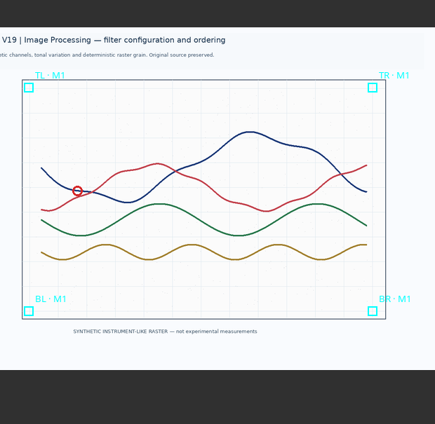
The configuration contains a four-corner calibration, with X from 0 to 10 seconds and Y from −20 to 80 millivolts, and a series with one manual point. These elements make it possible to tell changes to the pipeline apart from changes to the scientific data.
2. Opening Image Processing
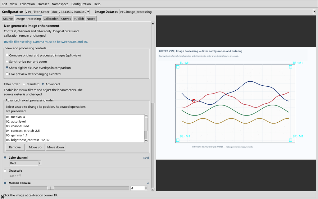
Select Image Processing in the Viewer tab bar or use View → Image Processing…. At the top of the panel there is the reminder Non-geometric image enhancement: the available filters act on contrast, intensity and channels, not on rotations, translations or distortions.
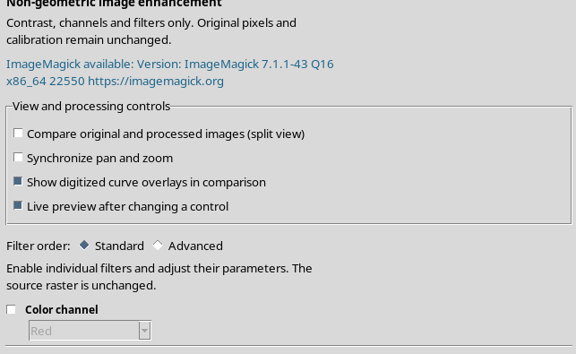
The left side contains the commands, while the Canvas on the right shows the image; the layout can change when side-by-side comparison is turned on.
3. The Scrollable List of Filters
The operations are shown in separate rows. Each row has a checkbox that enables the filter and, where applicable, a choice from a menu, a slider or a numeric field.
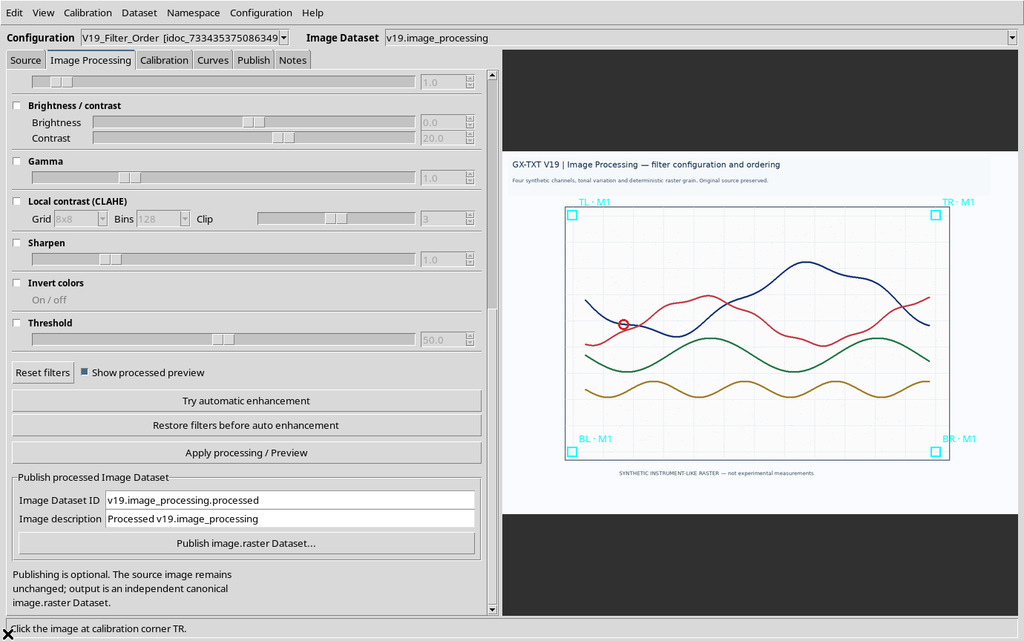
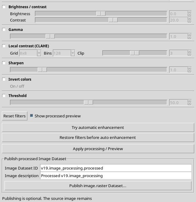
The parameters state how a filter will work; the checkbox decides whether that filter takes part in the pipeline. A disabled numeric control does not correspond to an active operation.
4. The Lower Commands of the Panel
Scrolling down you find Reset filters, Try automatic enhancement, Restore filters before auto enhancement, Show processed preview, Apply processing / Preview and the Publish processed Image Dataset area.
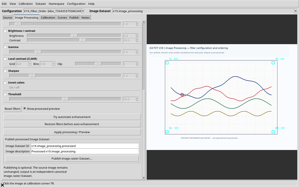
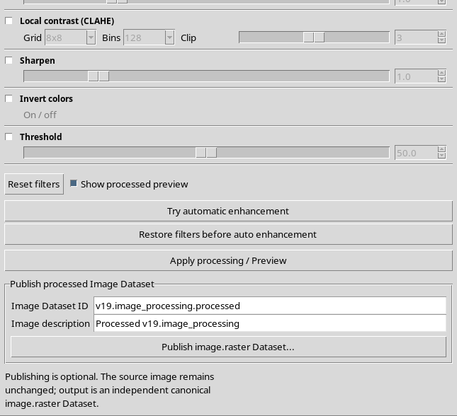
These are different operations: choosing filters, generating a preview and publishing a Dataset must not be confused. In particular, having a configured pipeline does not mean that a processed raster has already been created.
5. Checking the ImageMagick Engine
GX-TXT uses ImageMagick for processing. The availability of the engine is reported at the top of Image Processing. If the engine is not configured, the other Digitalizer commands remain usable, but the result of the filters cannot be obtained.
The engine is configured through GX-TXT Configuration → Runtime → ImageMagick. There is no need to set arbitrary paths directly in the filter list.
6. Turning Off Live Preview During Preparation
The Live preview after changing a control command requests a new processing run after a filter is changed, when the engine is available. The request is briefly deferred to avoid recomputing at every small slider movement.
To prepare a pipeline calmly, temporarily turn off Live preview.
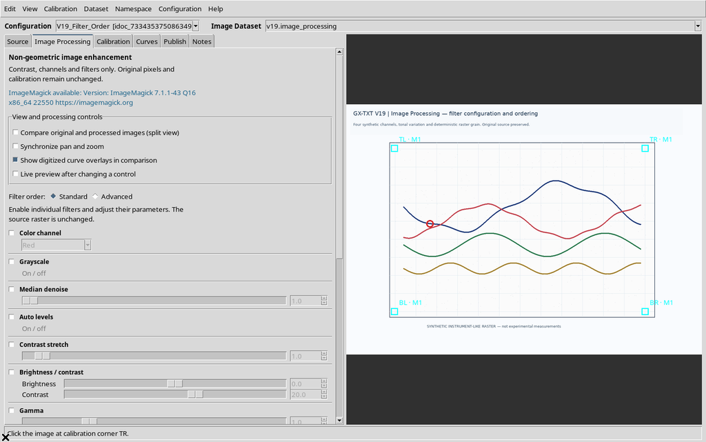
The operations are updated in the configuration even when no new preview is generated. Apply processing / Preview stays distinct from editing the field.
7. Enabling a Numeric Parameter: Gamma
A numeric filter has a value that can be changed with the visible control. For example, Gamma acts on the non-linear relationship between input intensity and output intensity; it does not change the pixel coordinates.
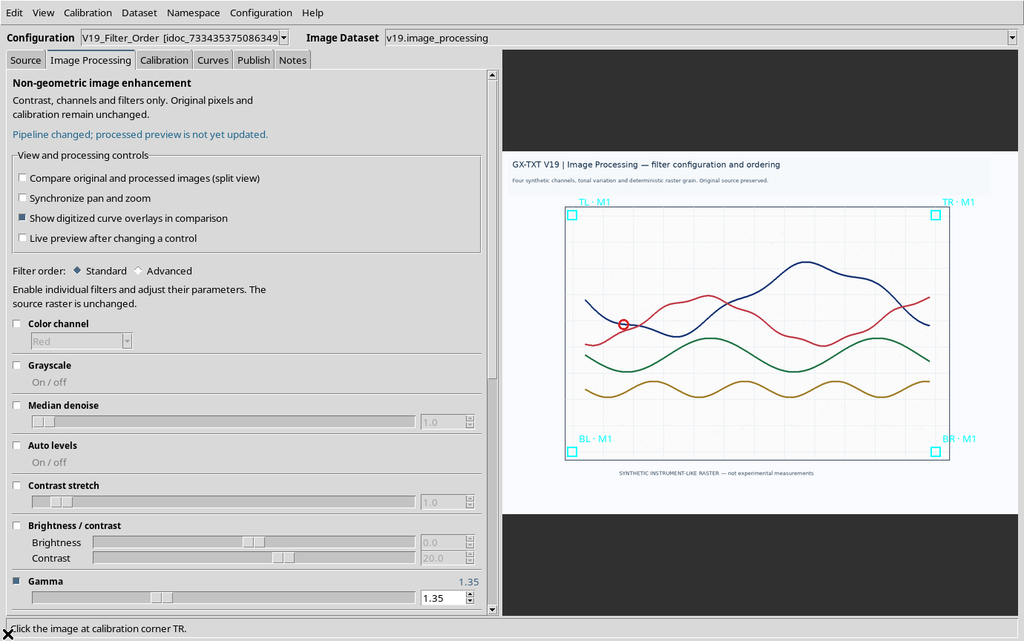
The chosen number becomes part of the active operation. To verify a scientific result, you need to note both the filter type and its value.
8. Color Channel and Grayscale in Standard
In Standard mode, Color channel and Grayscale are alternatives: the first selects a component of the image; the second removes the color differences.
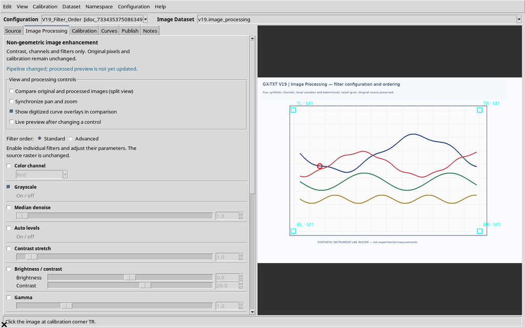
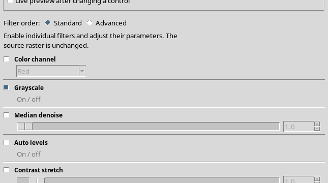
Enabling Grayscale removes a previous Color channel operation from the Standard sequence. It therefore makes no sense to assume that both act at the same time in this simple mode.
9. Selecting a Color Channel
For Color channel the choices are Red, Green, Blue and Luminance. Choose the channel in which the trace to be recognized stands out most from the grid or the other curves.
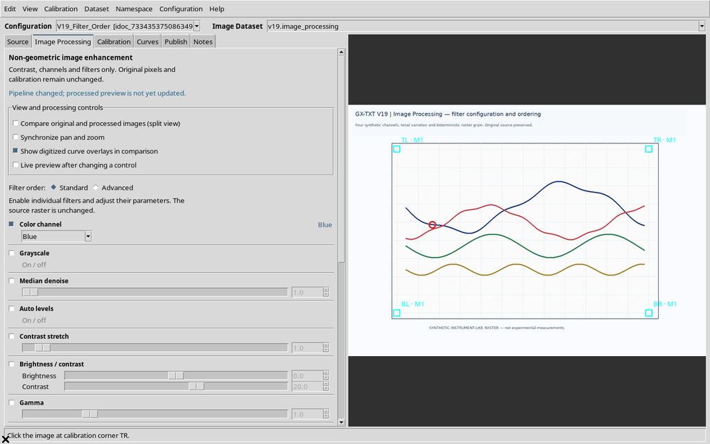
A channel can improve the contrast of one curve and worsen that of another. The choice must depend on the real color of the stroke and on the purpose of the digitization, not on a universally correct default value.
10. Enabling and Disabling a Filter with a Parameter
The Median denoise filter attenuates very small local features through median processing controlled by the radius. If the checkbox is disabled, the filter no longer appears among the actual operations.
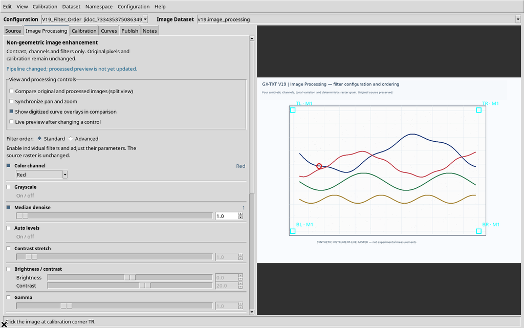
In the Viewer version examined, after disabling and re-enabling a numeric filter you need to check its parameter again: some settings may go back to the default value. The checking procedure is illustrated later with Gamma.
11. Building a Standard Pipeline with Several Operations
Enable the necessary filters with their checkboxes. In the demonstration configuration ten filters are active; Grayscale stays disabled because Color channel is enabled.
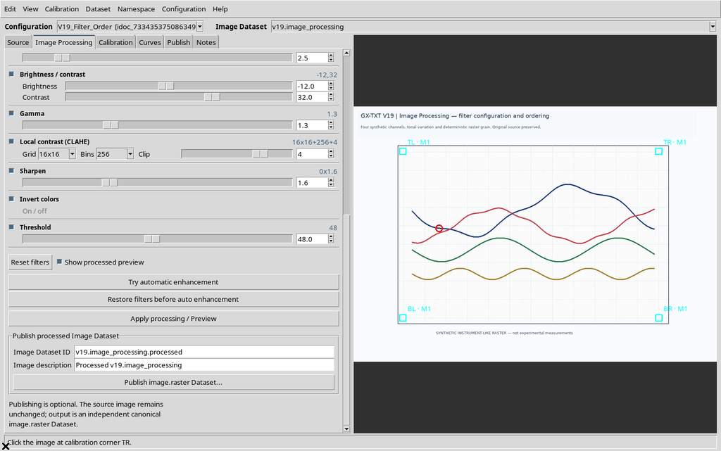
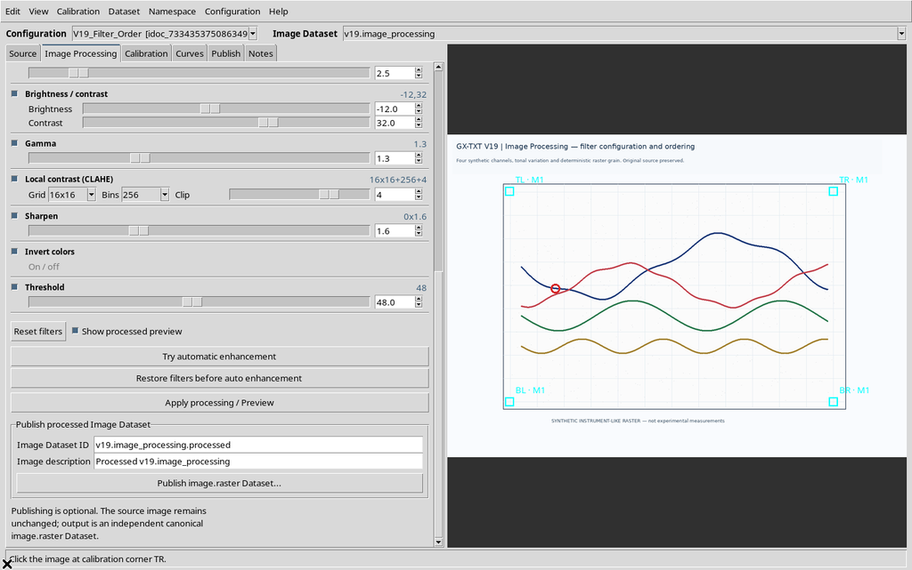
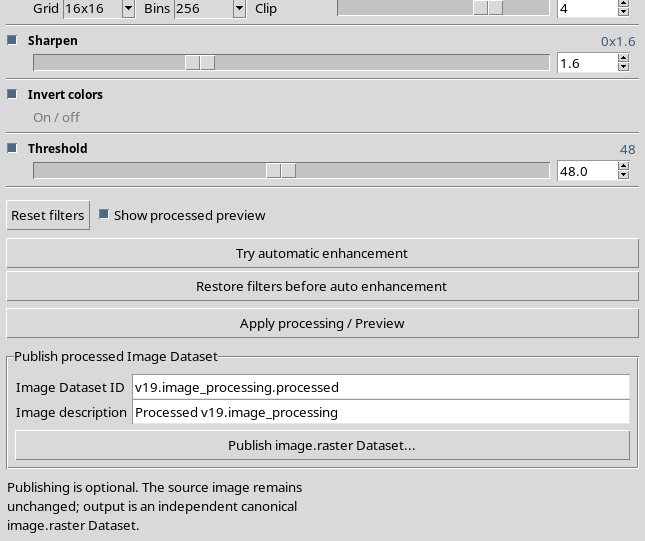
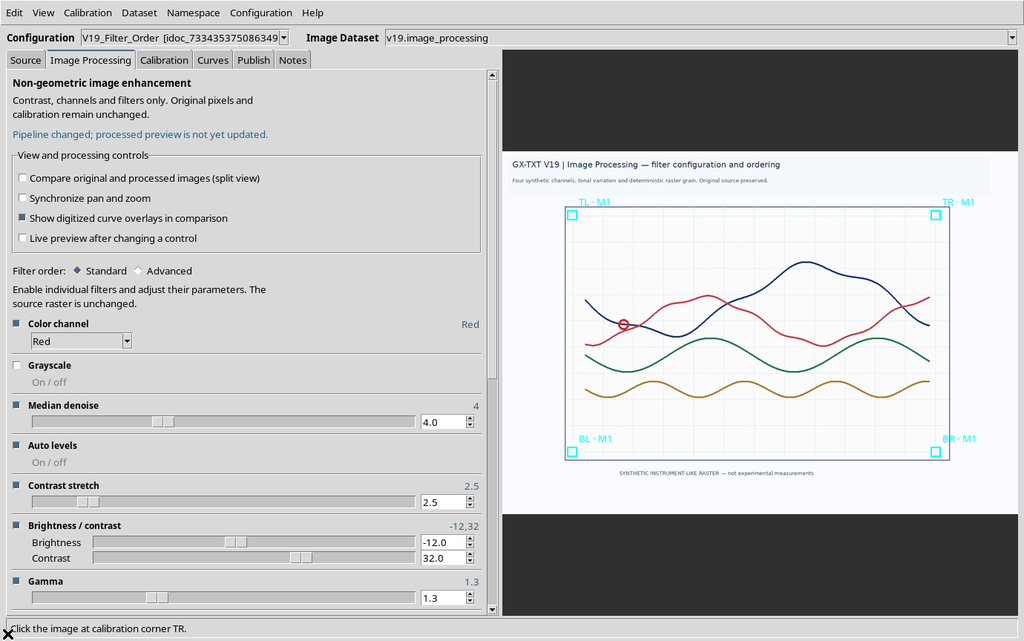
There is no need to use all the filters in real work. A short, scientifically motivated pipeline is often easier to check, document and reproduce than a long chain of processing steps.
12. How Standard Determines the Order
Standard sorts the filters according to a fixed sequence, independent of the order in which the user enabled them:
| Position | Operation |
|---|---|
| 1 | Color channel |
| 2 | Grayscale |
| 3 | Median denoise |
| 4 | Auto levels |
| 5 | Contrast stretch |
| 6 | Brightness / contrast |
| 7 | Gamma |
| 8 | Local contrast (CLAHE) |
| 9 | Sharpen |
| 10 | Invert colors |
| 11 | Threshold |
Operations that are not enabled are skipped; in practice Standard keeps only the rows actually selected. This sequence is a reasonable starting point, not a guarantee of optimal quality.
13. Switching to Advanced
Selecting Advanced under Filter order shows the Advanced · exact processing order frame, with a numbered list of the actual steps.
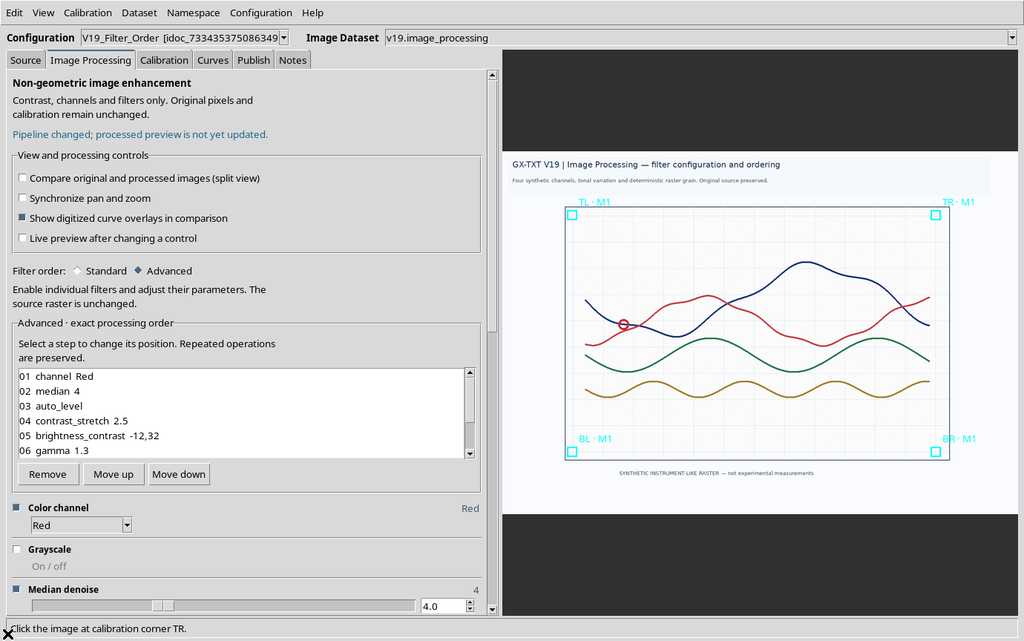
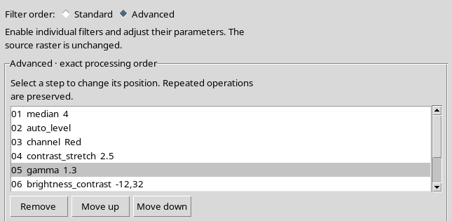
In the list, each row shows position, filter type and value. The list is distinct from the checkboxes: it describes the processing sequence, not the fixed list of all available controls.
14. Move Up and Move Down Change the Pipeline
Select a row and press Move down or Move up. For example, moving Color channel below Median denoise, the order no longer matches the one imposed by Standard.
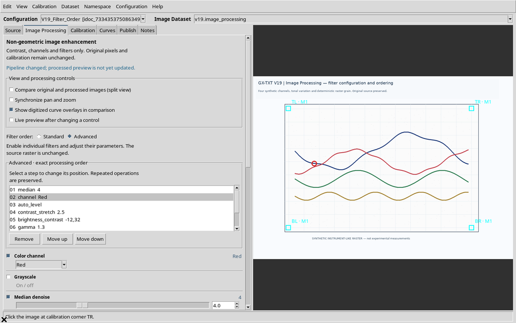
Further moves can change the sequence again.
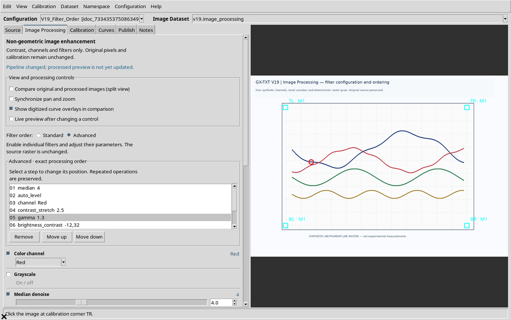
Changing the order is scientifically significant because many photometric operations do not commute: applying A and then B is not necessarily the same as applying B and then A.
15. Movement Limits and Remove
The first step cannot be moved further up and the last cannot be moved further down. These attempts leave the pipeline unchanged.
The Remove button deletes the selected operation from the list.
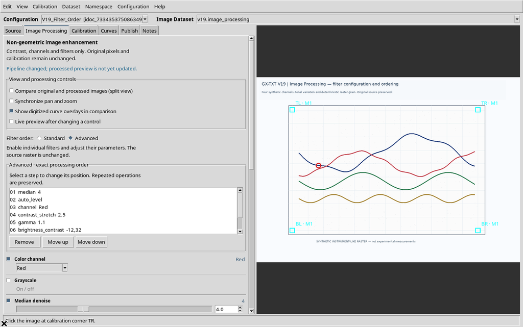
Its checkbox is disabled and the other operations remain. If the filter is later re-enabled in Advanced, it may be added at the end of the list; check the order and the parameter again.
16. Out-of-Range Parameters: Median Denoise
The radius of Median denoise ranges from 1 to 10. Entering 11, the Viewer reports that the value is invalid.
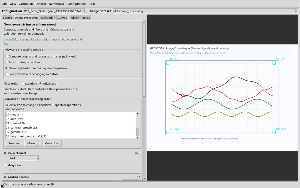
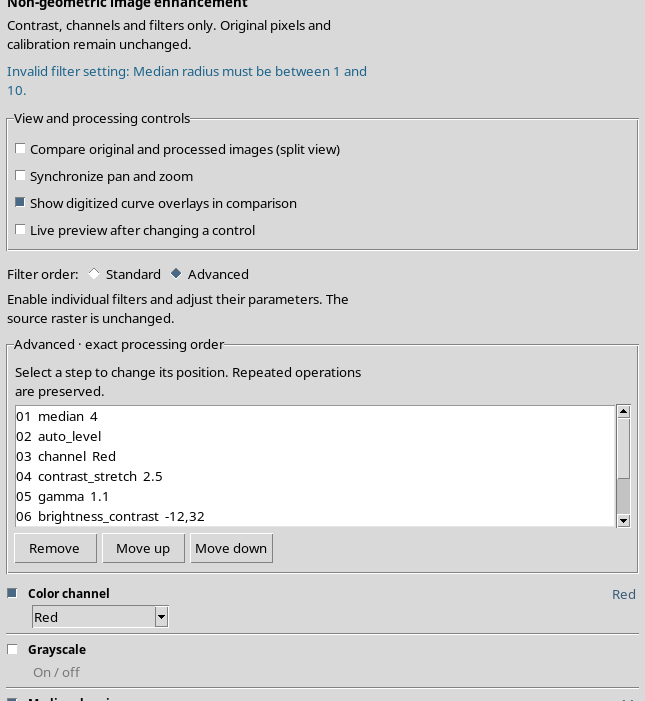
The recorded operation keeps the previous valid value. Do not mistake the invalid number still visible in the field for the parameter actually accepted in the list.
17. Out-of-Range Parameters: Gamma
Gamma validation requires a value between 0.05 and 10. Entering 0, the Viewer rejects the change.
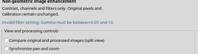
Here too the invalid number must not be considered part of the pipeline. Correct the field with an allowed value and check the row in the list before applying the processing.
18. Going Back to Standard
When switching explicitly from Advanced to Standard, the Viewer reorders the operations according to the default sequence.
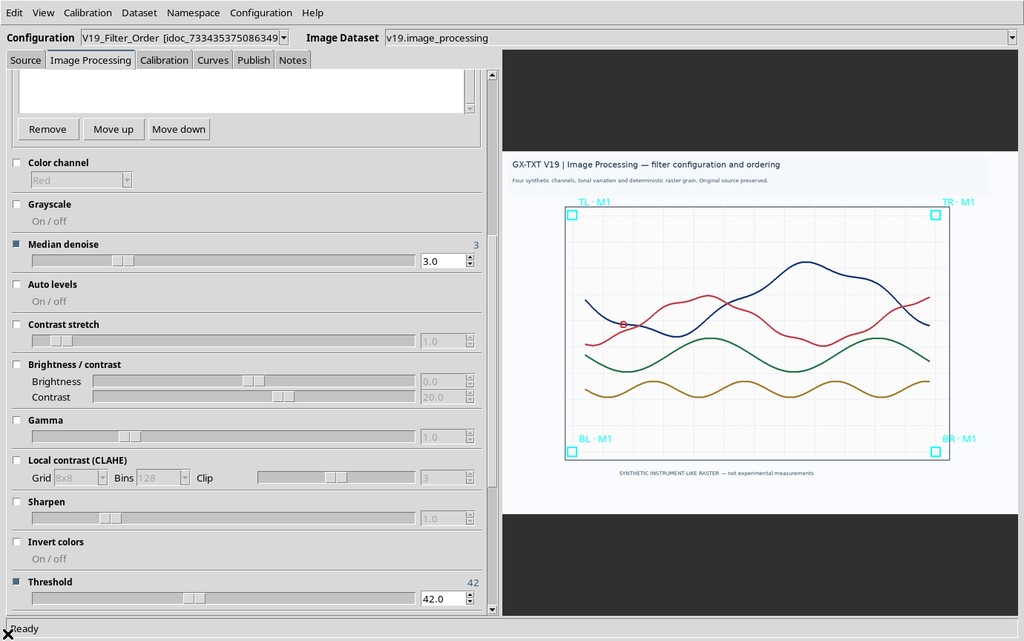
This operation should not be done carelessly when the Advanced order was chosen for a precise scientific purpose. The final result depends not only on the values but also on their order.
19. The Advanced List Is Reversible
In Advanced, a filter can be moved up and later returned to its previous position.
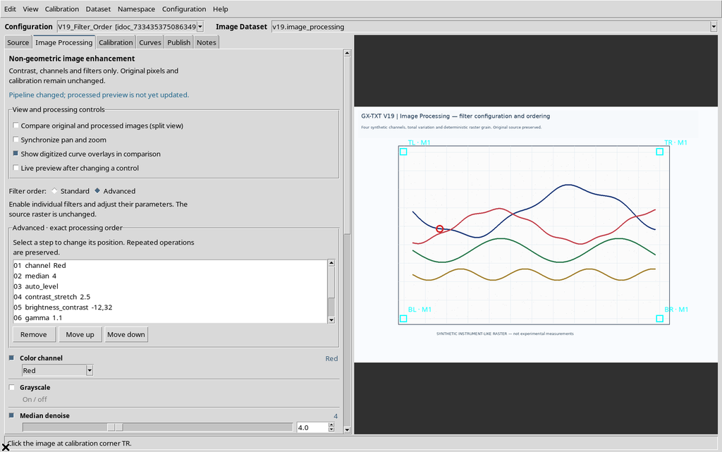
In the example, two opposite moves rebuild the previous sequence, without losing the parameters of the operations that stayed enabled.
20. Reset Filters: Clearing the Pipeline
Reset filters deletes all the configured processing operations.
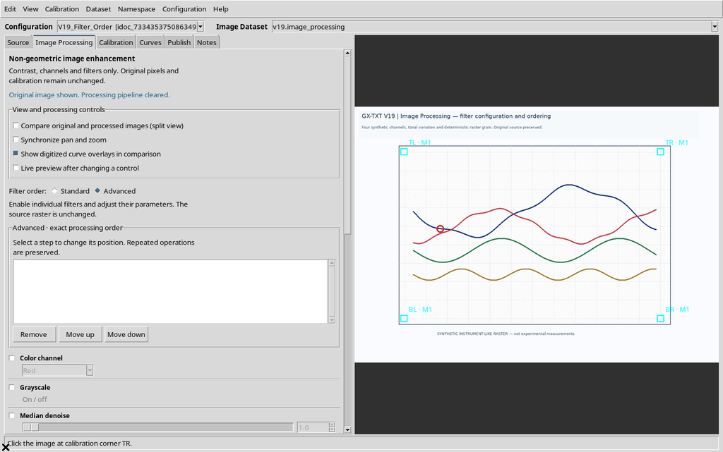
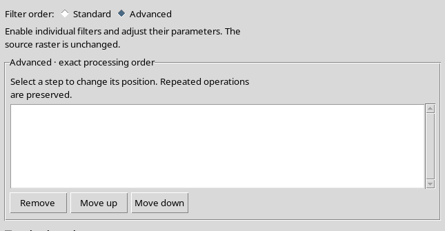
The original raster is not deleted and the manual point of the curve stays in place. Reset is useful when you want to redesign the filters starting from a state with no active operations.
21. Building an Essential Advanced Pipeline
A deliberately non-Standard example uses three operations in this order:
Gamma 1.8 → Threshold 42 → Median 3
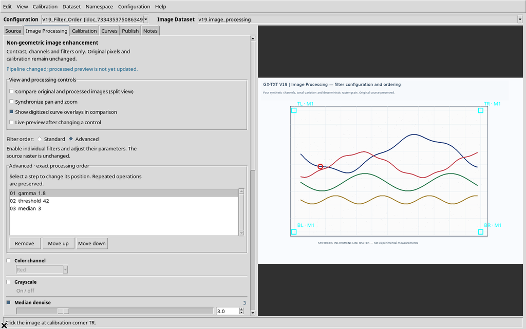
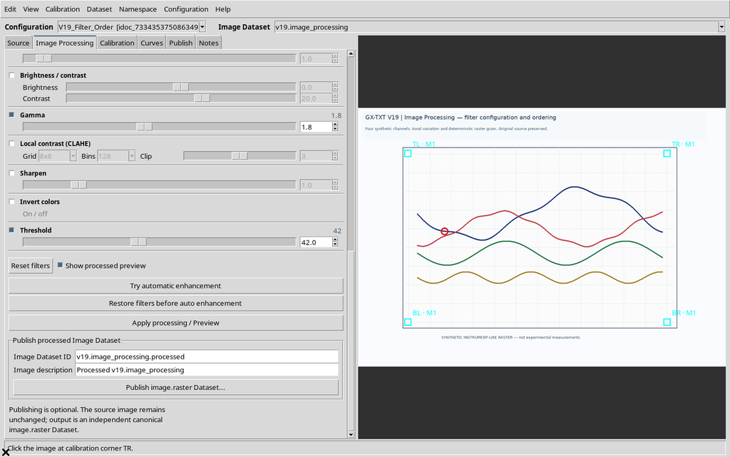
The Advanced list makes the order explicit. In Standard the same filters would be ordered Median → Gamma → Threshold. The two orders do not necessarily represent the same processing.
22. Why the Order Matters
Gamma changes intensities non-linearly; Threshold separates the levels with respect to a threshold; Median acts on the local result. If a threshold is applied before a tonal transformation, the decision to classify a pixel can change.
For this reason a reproducible pipeline requires names, parameters, order and source. It is not enough to write that an image was simply enhanced.
23. Saving the Configuration
After checking the order and all the values, use Configuration → Save configuration.
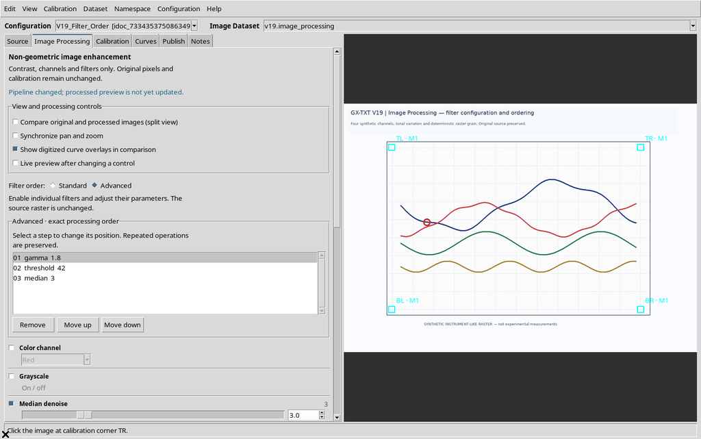
The parameters and the sequence of operations are saved in the Viewer configuration. This step must not be confused with publishing a new Image Dataset, nor with the corresponding preview having already been produced.
24. Reopening in the Same Session
Close the Viewer normally, reopen it from the Session and go back to Image Processing.
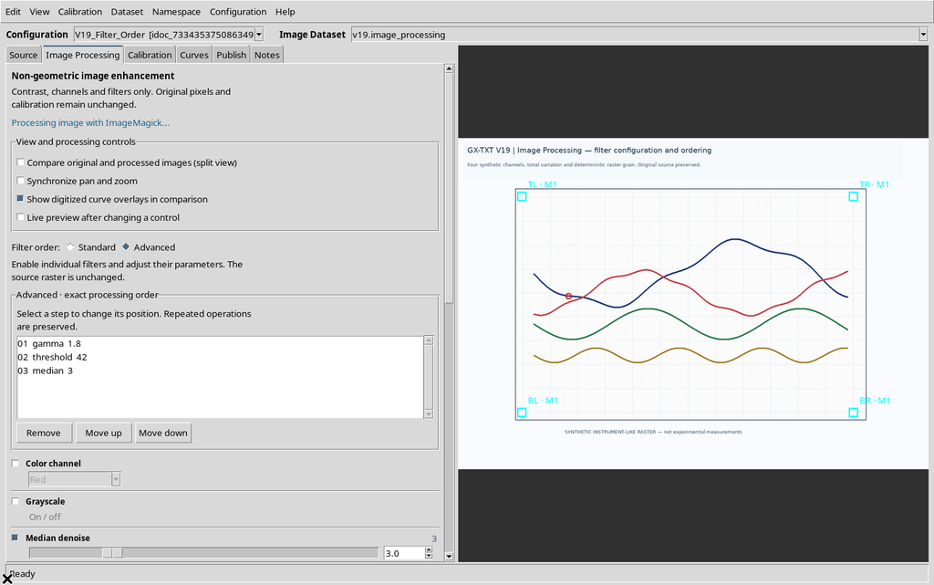
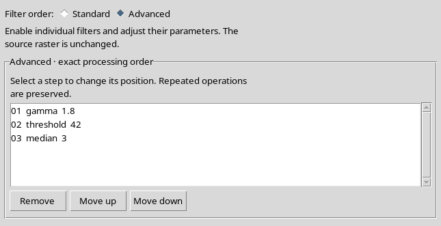
In the example, Gamma 1.8 → Threshold 42 → Median 3 is recovered, still in Advanced, together with the disabled Live preview preference. The persistence of the order makes it possible to reconstruct the preparation of the future processing.
25. Image Processing Is Not the Point Editor
The Image Processing tab lets you prepare an image, not edit scientific records by clicking on the Canvas. Manual editing of points takes place in the Curves tab.
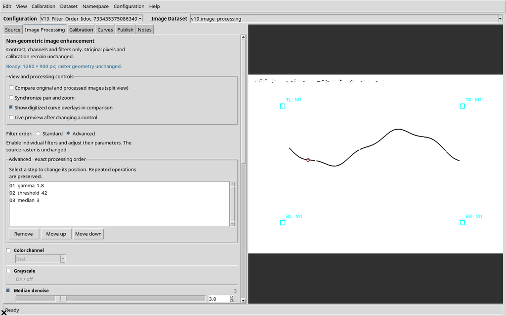
A click on the image and the Delete key, while Image Processing is active, neither add nor remove points of the series. The calibration and the source keep the same coordinates.
26. Checking the Value Before Disabling Gamma
Suppose an Advanced pipeline contains Gamma = 1.8.
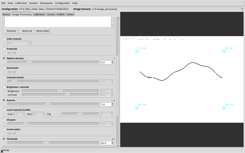
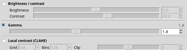
Before using the On/Off button, it is useful to check the value in the row and in the actual sequence, so that it can be restored if needed.
27. Disabling Gamma Can Restore the Default Value
In the version examined, disabling Gamma changes its numeric control from 1.8 to 1.0, which is the default value.
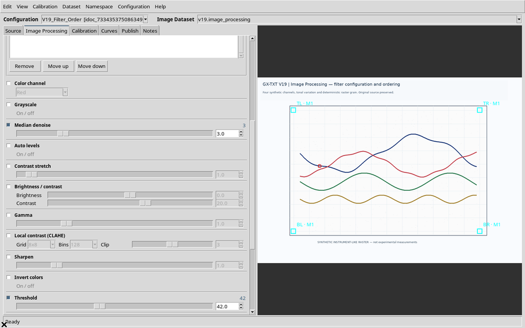
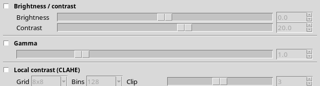
This is a limitation to keep in mind: disabling the filter does not currently guarantee that the previously chosen parameter is kept.
28. Re-enabling Gamma Does Not Recover the Number
When Gamma is re-enabled, the row still shows 1.0 instead of 1.8.
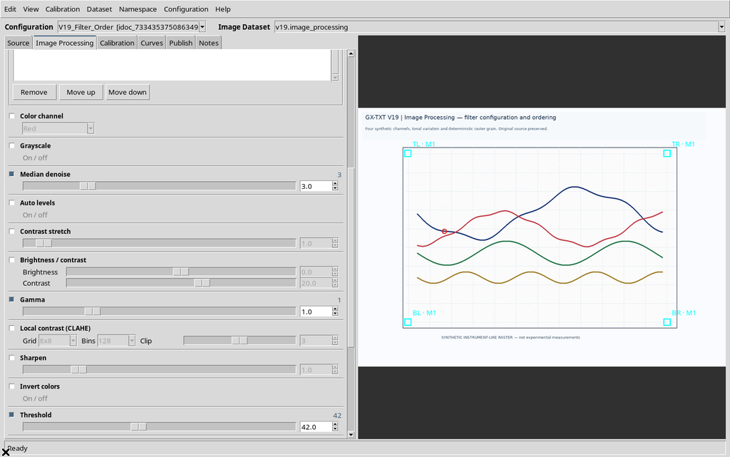
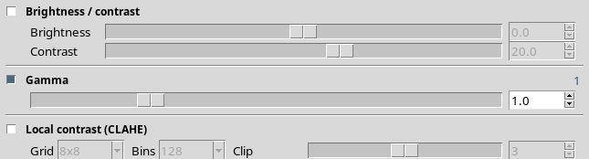
The same kind of parameter loss was found with Median denoise. Before generating a new preview, set the desired value again and check the order of the operations, especially when Advanced mode is active.
29. Restoring Value and Order
To recover the desired sequence, set Gamma 1.8 again and move it to the intended position with the Advanced controls.
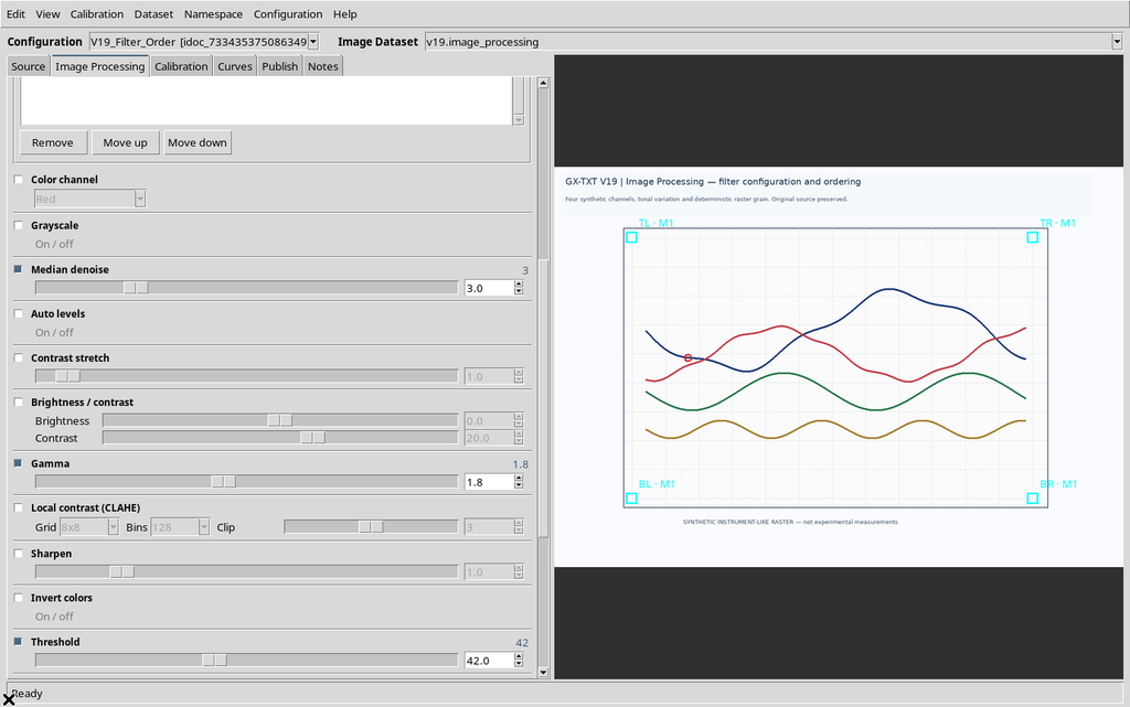
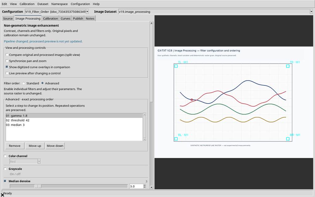
Check the whole pipeline before saving. This avoids mistakenly using a filter with a default parameter instead of the one motivated for the image under examination.
30. Reference of the Available Filters
| Filter | Parameter | Main use |
|---|---|---|
| Color channel | Red, Green, Blue, Luminance | Isolate a color component |
| Grayscale | On / off | Reduce to gray levels |
| Median denoise | Radius 1–10 | Reduce local noise |
| Auto levels | On / off | Expand the tonal range |
| Contrast stretch | Percentage 0–20 | Reduce the influence of the distribution tails |
| Brightness / contrast | Two values −100…100 | Adjust brightness and contrast |
| Gamma | Positive value, validated 0.05–10 | Non-linear tonal transformation |
| Local contrast (CLAHE) | Grid, bins, clip | Local contrast |
| Sharpen | Sigma 0.1–4.9 | Increase the apparent sharpness of edges |
| Invert colors | On / off | Invert the levels |
| Threshold | Percentage 0–100 | Separation by threshold |
For CLAHE, the available grids are 2×2, 4×4, 8×8, 16×16 and 32×32; the available bins values are 64, 128 and 256, while clip takes integers from 1 to 5. The Sharpen control accepts the internal parameter in the form 0xSigma, for example 0x1.6.
These settings are processing tools; they are not equivalent to scale corrections or scientific measurements. The parameters must be chosen according to the original quality of the image.
31. Comparison, Preview and Automatic Suggestion
The panel also offers Compare original and processed images (split view), Synchronize pan and zoom, Show digitized curve overlays in comparison and Show processed preview. These options concern the display and do not replace the choice of filters.
The Try automatic enhancement button proposes a possible enhancement sequence; Restore filters before auto enhancement lets you recover the previous configuration, when available in the current configuration and source. An automatic proposal must not be considered valid without a visual comparison.
The Apply processing / Preview command is used to generate the processed image to be examined. Handling the two Canvases and checking the images produced will be covered in the guide devoted to the preview.
32. Getting Ready to Use the Results
Before applying a real processing:
- Check the source and the calibration; do not alter the original geometry.
- Identify the visual problem to correct: channel, noise, local contrast, gamma or threshold.
- Choose a limited number of filters with motivated parameters.
- Use Standard as a starting point, or Advanced when the order is an essential part of the method.
- After every re-enabling, check that the numeric values have not gone back to the defaults.
- Confirm the order and save the configuration.
- Generate and evaluate the preview before relying on the processed trace for a digitization.
- Publish a new Dataset only when the processed version has been checked and must be kept separately.
The pipeline does not destroy the original image. However, a more contrasted image is not necessarily more faithful to the data: a filter can remove a faint part of the line, change the apparent edge or emphasize an artifact. For scientific digitization, the reference always remains the original raster together with the documented calibration.