

Declaring Uncertainties and Physical Covariance
In GX-TXT, digitizing a curve means deriving scientific points from the pixels of a calibrated image. The coordinates obtained do not automatically carry information about their uncertainty: the mere fact that the image has a given resolution or a visible thickness does not make it possible to establish how uncertain a measurement is.
Curve Digitalizer distinguishes no declared uncertainty, explicitly assigned physical standard uncertainties and numerically propagated localization and calibration uncertainties. This guide illustrates the difference between them and shows how to read the results of CURVE_DIGITIZER_UNCERTAINTY_API_v1, the NUMERIC_API_v1 numerical service and the published full covariance.
All the uncertainty values used in the example are teaching assumptions. They do not come from instruments, experimental repetitions or calibration certificates.
1. First Distinction: Points, Thickness and Uncertainty
Digitized points have a position in the raster and, after calibration, an X/Y position in physical units. The width of the line and the observations of the Quality report concern instead the graphic stroke. Neither of the two is a standard uncertainty.
Without a justified declaration, the system must not automatically introduce an error of one pixel, of half a pixel or a statistical spread estimated only from the appearance of the figure.
2. Synthetic Source and Calibration
The example uses an original raster of 1280 × 900 pixels, with a dark wavy line and a second, pink trace, deliberately kept apart. 15 manual points were acquired on the first line.
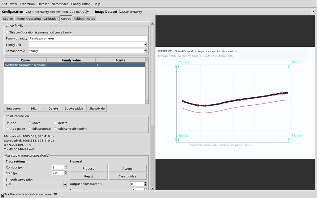
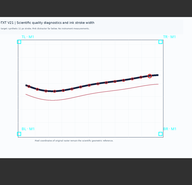
The four-corner calibration maps X to 0–10 s and Y to −20–80 mV. The same coordinates, the same point order and the same identifiers will be kept in the three numerical Datasets used for comparison.
3. Publishing Without Uncertainty: Error Model None
In Publish, select the accepted calibration and prepare a new numerical Dataset.
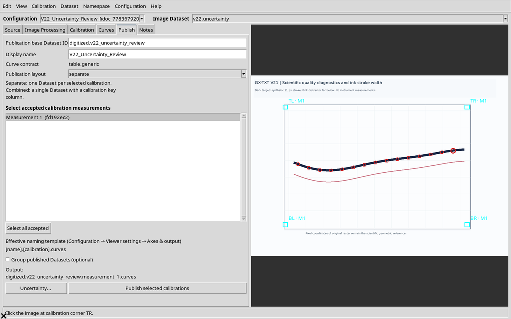
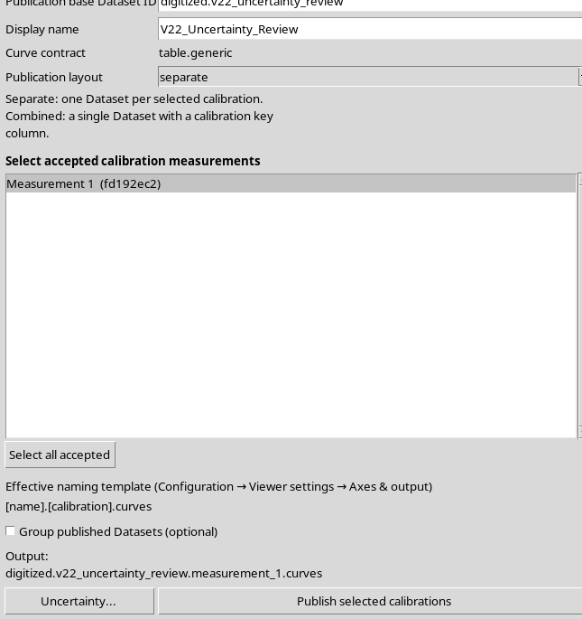
With the none model, the Publish selected calibrations command creates the ordinary table with the scientific and raster coordinates.
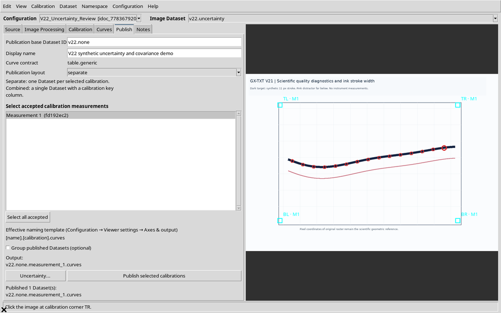
The table in this example contains 15 rows and does not contain the sigma_x, sigma_y and covariance_xy columns. The absence of these columns does not mean that the measurement is exact; it means that no metrological model has been declared.
4. Opening Pixel and Calibration Uncertainty
From Publish, press Uncertainty… to open the declaration editor.
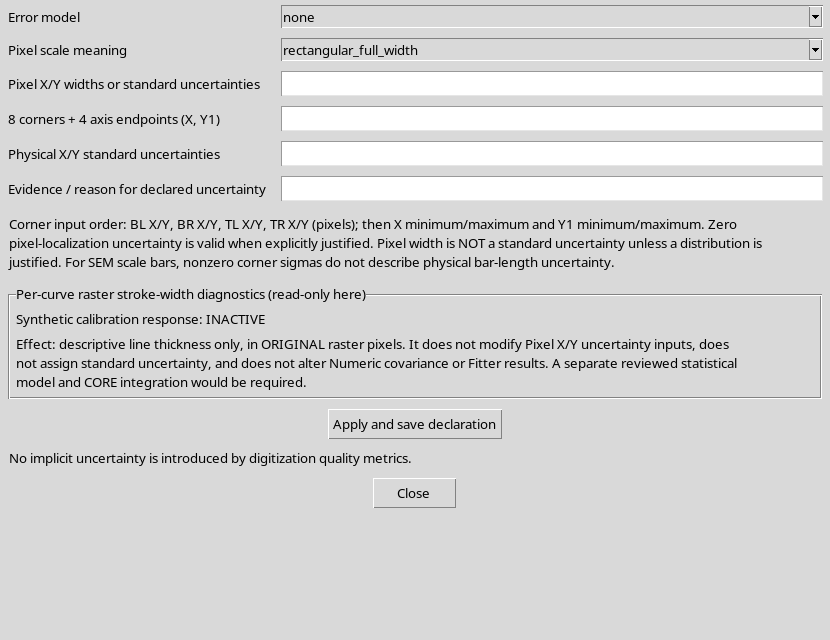
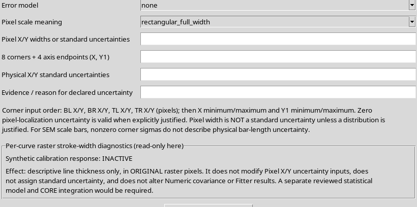
At the start Error model = none is selected. The fields for pixels, calibration inputs and physical uncertainties are empty. No pre-filled statistical values appear.
The editor stores scientific assumptions in the current configuration: it is not a simple graphic control of the Canvas.
5. The Three Available Models
The Error model choice offers three modes:
| Model | Meaning |
|---|---|
| none | No declared uncertainty is propagated |
| physical_override | Physical X and Y standard uncertainties are given directly |
| pixel_calibration | A pixel localization model and the uncertain calibration inputs are given |
This is not a ranking of data quality. Each model is admissible only if the operator can justify its assumptions.
6. Physical_override: Assigning Two Physical Sigmas
Choose physical_override and enter two standard uncertainties in the physical units of the axes. In the example 0.03 s and 0.20 mV are declared.
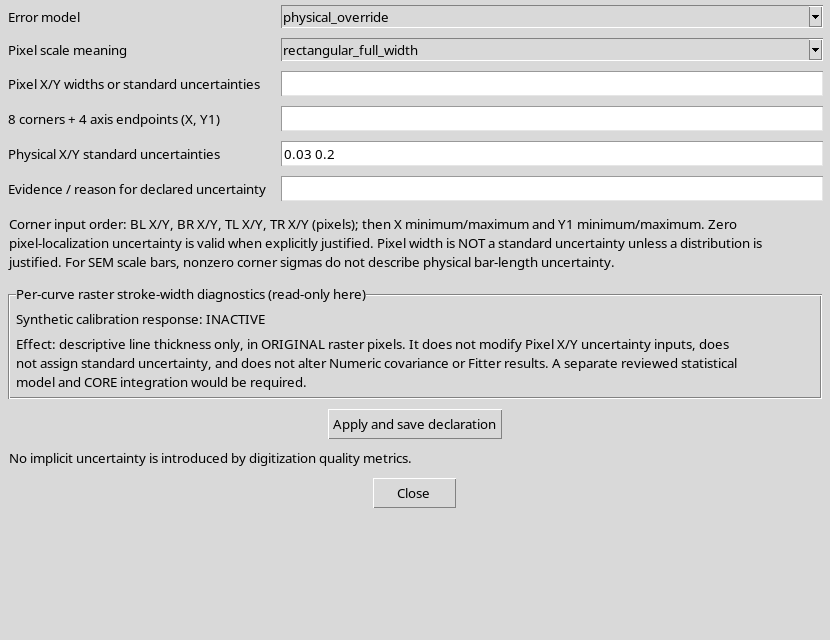
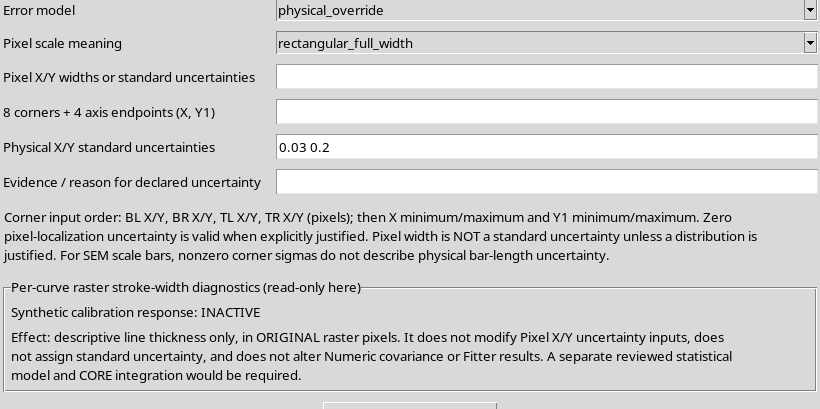
These are hypothetical numbers to show how the software works; they are not a real characterization of the synthetic signal, of time or of the measured amplitude.
7. The Justification Is Required
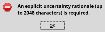
This safeguard prevents a declaration from being recorded without the context needed to interpret it.
8. Confirming the Physical Declaration
Enter an explicit justification, check the units and press Apply and save declaration.
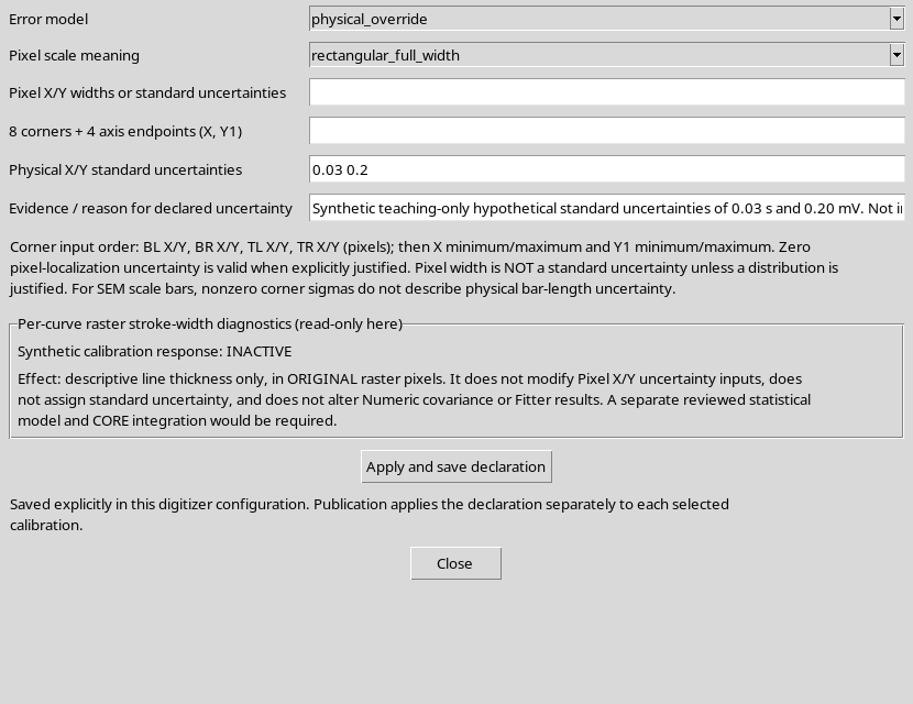
The window status shows that the declaration has been saved in the configuration. The two numbers are now a reviewed scientific assumption, not a temporary interface setting.
9. Publishing the Physical_override Model
Close the editor, enter a distinct Dataset ID and publish the accepted calibration.
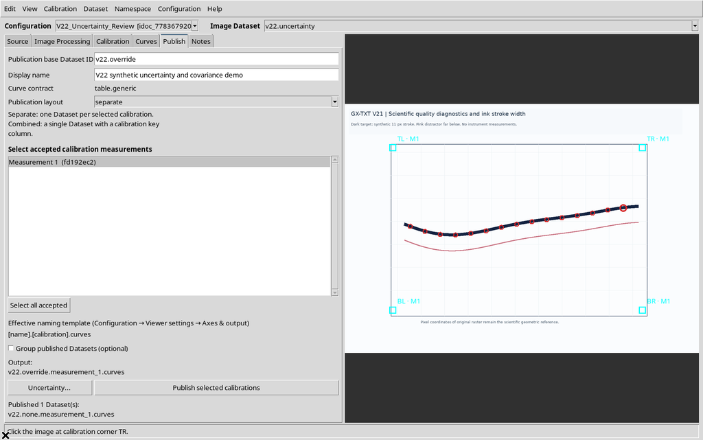
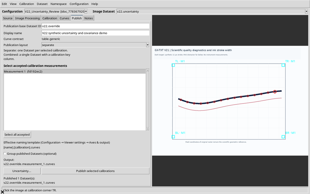
The result contains the sigma_x, sigma_y and covariance_xy columns, with the declared standard values. In the example all points have sigma_x = 0.03 s, sigma_y = 0.20 mV, and zero X/Y covariance.
10. Why Physical_override Does Not Create Shared Correlations
In the model declared here, the uncertainties are assigned independently to the physical coordinates of each point. No common contributions arising from the calibration are introduced.
The covariance matrix of the Y response is therefore diagonal, with a variance of 0.04 mV² for each point. The fact that the model is simple does not mean it is preferable: it is appropriate only if the assumed independence is scientifically tenable.
11. Reusing a Saved Declaration
Reopening Uncertainty…, the physical model just approved is reloaded.
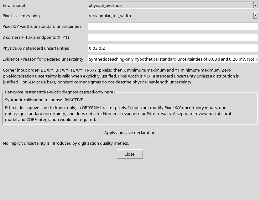
This makes it possible to check which assumptions are actually linked to the configuration. Changing one of its inputs does not retroactively change the Datasets already published.
12. Pixel_calibration: The Most Detailed Model
The pixel_calibration mode separates the uncertain localization of points on the raster from the uncertainties of the elements used to determine the calibration transformation.
For the single-axis configuration of the example, the editor requires two pixel inputs and twelve calibration standard uncertainties. The first concern the local position of the point, while the twelve can produce effects shared by several points.
13. Order of the Twelve Calibration Inputs
In the single-axis model the required order is:
| Indices | Origin of the standard uncertainties |
|---|---|
| 1–2 | Bottom left: pixel X, pixel Y |
| 3–4 | Bottom right: pixel X, pixel Y |
| 5–6 | Top left: pixel X, pixel Y |
| 7–8 | Top right: pixel X, pixel Y |
| 9–10 | X minimum, X maximum in X-axis units |
| 11–12 | Y minimum, Y maximum in Y-axis units |
The units of the first eight elements are original pixels; those of the last four are physical. A list without this correspondence does not document a reproducible calibration.
14. The GUI Rejects a Wrong Number of Inputs
If only two values are entered in the calibration uncertainty box, the editor rejects the declaration because it requires exactly twelve.
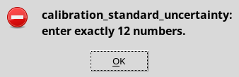
Missing parameters are not created implicitly and an incomplete matrix cannot be approved.
15. The GUI Rejects Negative Values
A standard uncertainty must be a finite, non-negative value. Entering a negative number in the list, the Viewer shows an error.
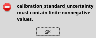
The check is distinct from the one on units and on the justification: the operator must ensure completeness, dimensional consistency and scientific meaning at the same time.
16. Explicitly Declared Zero Localization
The model accepts a pixel localization of 0 0, provided this choice is explicitly justified.
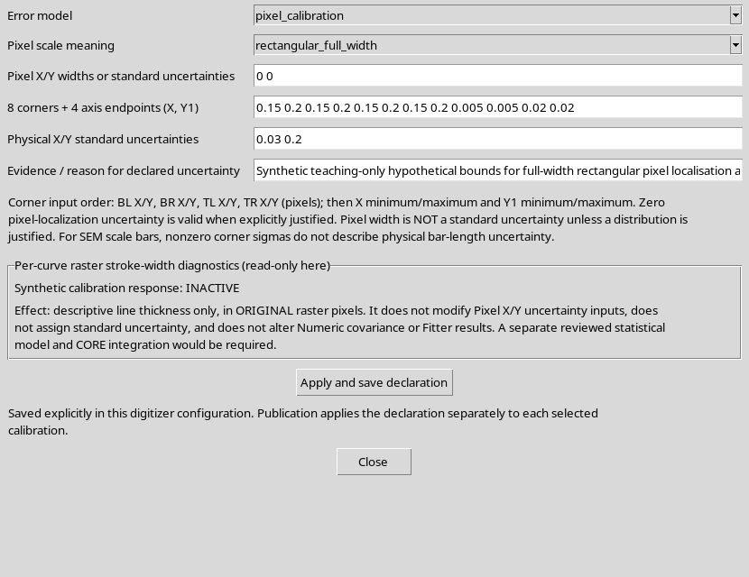
The example shows that the Viewer does not automatically impose a positive threshold derived from the pixel size. A zero localization does not, however, cancel the shared contributions of the twelve non-zero calibration uncertainties.
The zero value is a declared choice of the model: it does not imply that the real localization of the pixels is exact.
17. Rectangular Width and Standard Uncertainty
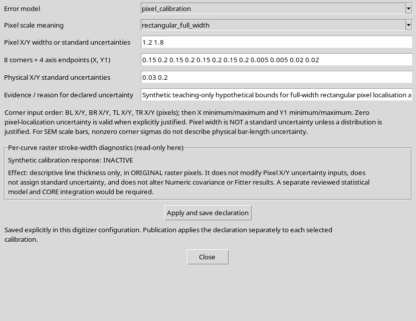
Selecting rectangular_full_width, the two localization numbers represent the full widths of uniform intervals, not standard deviations directly.
For a full width w, the declared conversion is:
σ_pixel = w / √12
In the example the widths 1.2 px and 1.8 px correspond to about 0.3464 px and 0.5196 px of local standard uncertainty.
18. Twelve Hypothetical Uncertainties for the Calibration
The eight pixel coordinates of the corners receive, for demonstration purposes, the alternating standard uncertainties 0.15 px in X and 0.20 px in Y. The X limits receive 0.005 s each; the Y limits 0.02 mV each.
These values were not measured. They serve to build an example in which the calibration transformation has a common, recognizable contribution to the covariance of several points.
19. Publishing the Correlated Model
After the justification and Apply and save declaration, go back to Publish and use a new Dataset ID.
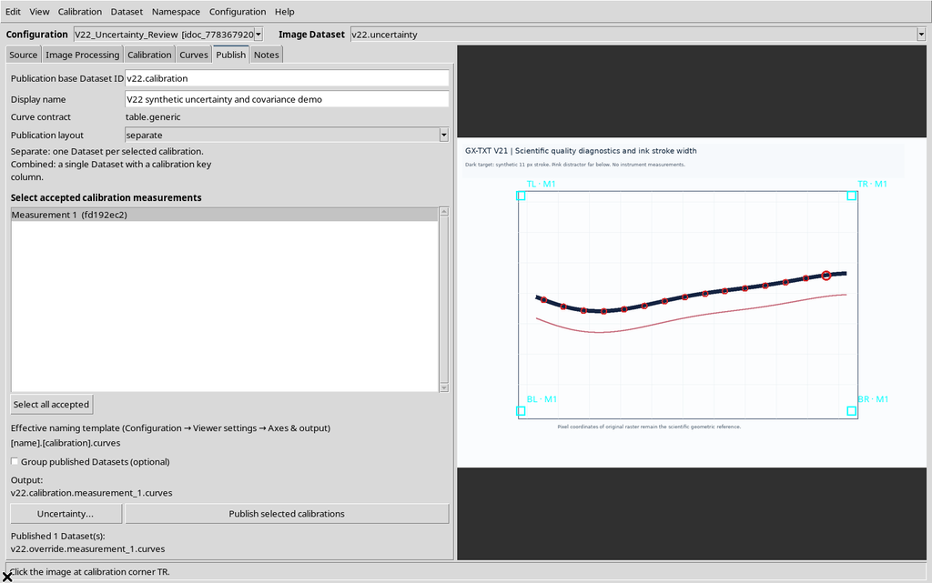
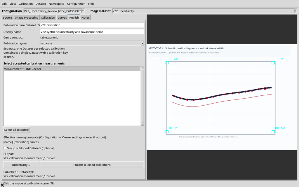
The 15 numerical rows keep the same identifiers, the same order and the same coordinates as the none and physical_override examples, but now contain uncertainties propagated by the public numerical service.
20. Comparing the Three Datasets
| Property | none | physical_override | pixel_calibration |
|---|---|---|---|
| X/Y coordinates | Unchanged | Unchanged | Unchanged |
| Published rows | 15 | 15 | 15 |
| Sigma/covariance columns | Absent | Present | Present |
| Shared calibration contributions | Not declared | Absent in the model | Present |
| Covariance between different points | Not published | Zero in the independent model | Generally non-zero |
A smaller marginal sigma does not prove a more accurate result if the assumptions that produced it are different.
21. Local and Shared Factors
The numerical model keeps two kinds of contributions: a factor Lᵢ associated with the individual point and a factor Sᵢ associated with the common inputs of the calibration.
The physical covariance between the coordinates of points i and j is:
Cov(zᵢ,zⱼ) = δᵢⱼ · LᵢLᵢᵀ + SᵢSⱼᵀ
The first term exists on the diagonal of the points; the second can produce a covariance even when i and j are different. This is why the sigma_x and sigma_y columns alone do not describe all the effects of the calibration.
22. Sigma_x, Sigma_y and Covariance_xy
For each point the result contains two marginal standard uncertainties, in the units of X and Y, and the covariance between its coordinates.
For the test the units are s, mV and s·mV. In the pixel_calibration model covariance_xy can also be non-zero, because the calibration inputs affect both scientific coordinates.
covariance_xy is not a dimensionless correlation, and must not be turned automatically into an independent weight for a fit.
23. What Covariance Between Points Means
When the same calibration determines the position of several points, its uncertainty can introduce coordinated movements in the resulting coordinates. The covariance between two distinct points records this dependence.
In the example, the rebuilt Y matrix has a maximum absolute off-diagonal value of about 0.000768 mV². This number concerns only the explicit teaching assumptions.
24. Changing a Point Makes the Review Obsolete
After the uncertainty review, if a sixteenth point is added to the curve, the saved declaration no longer describes exactly the same set of points and identifiers.
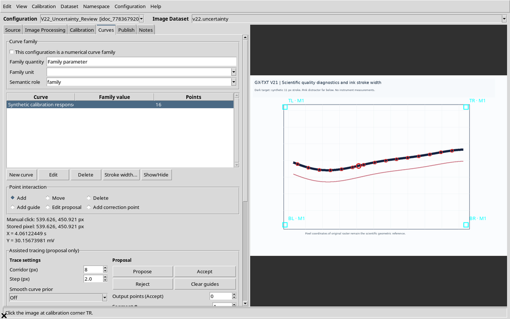
Trying to publish another Dataset without a new review, the GUI blocks the operation.
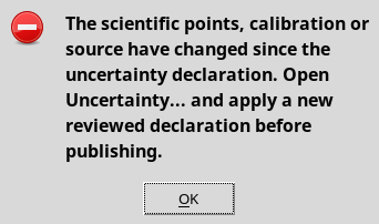
This safeguard prevents numerical factors computed for fifteen points from being silently assigned to a different Dataset.
25. Undo and Restoring the Data
With Edit → Undo you can restore the previous fifteen points.
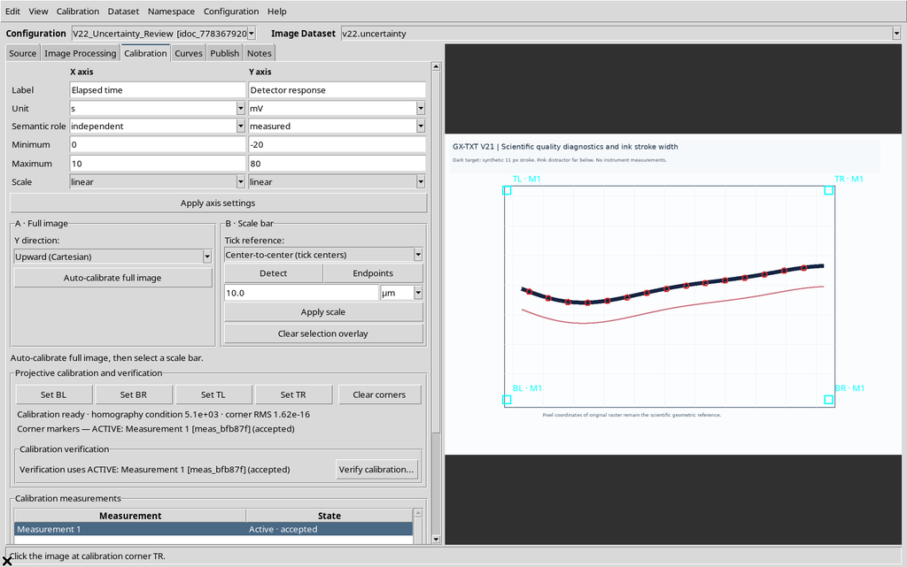
The Dataset published before the change stays unchanged in any case. The current review must be compared with the actual scientific state before a new publication.
26. Normal_standard_uncertainty Is a Second Convention
The Pixel scale meaning menu also offers normal_standard_uncertainty. In this mode the number entered directly represents a standard localization sigma, not the full width of a rectangular interval.
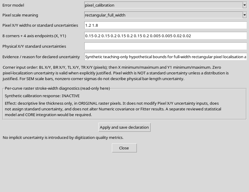
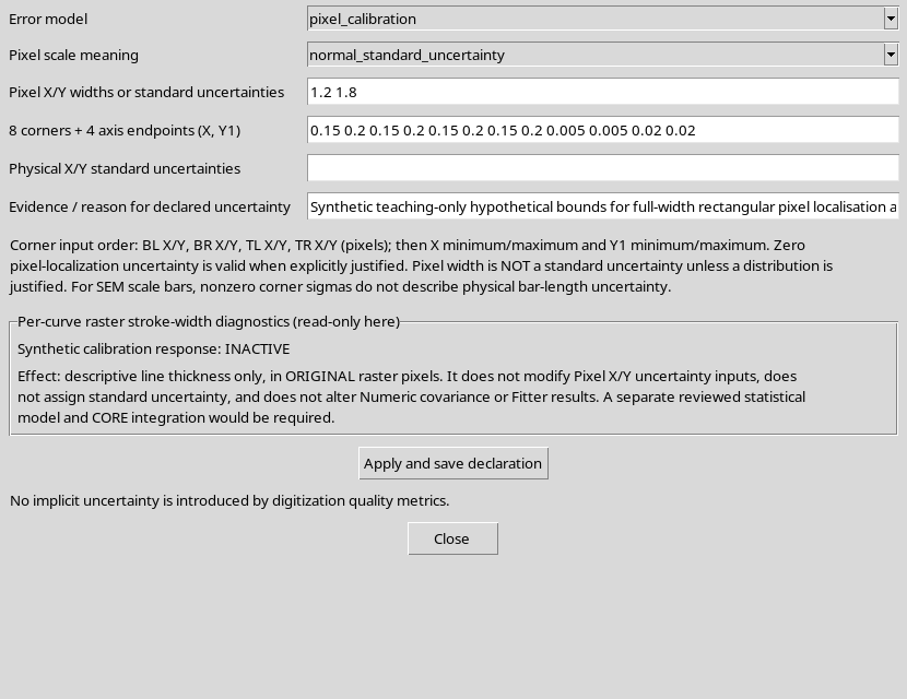
If the choice is changed without pressing Apply and save declaration, reopening the editor still shows the previously approved rectangular model.
Changing the convention without changing the numbers can completely alter their meaning: it must be treated as a new scientific declaration.
27. Save, Close and Reopen
Save the configuration, close Curve Digitalizer normally and reopen it in the same Session.
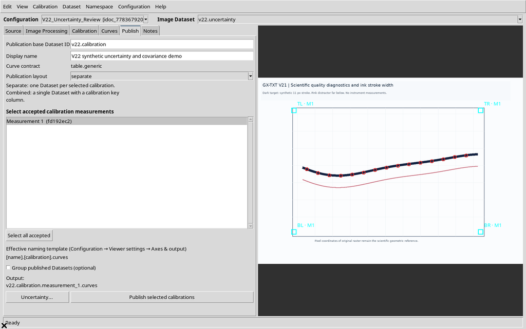
The declaration stays available in the document.
Reopening kept the fifteen points, the calibration, the identity of the source and the pixel_calibration model with the declared numerical assumptions.
28. Viewing the Numerical Data in the CORE Viewer
A published Dataset can be opened from the GX-TXT browser with the CORE Scientific Dataset Viewer, without accessing the private objects of Curve Digitalizer.
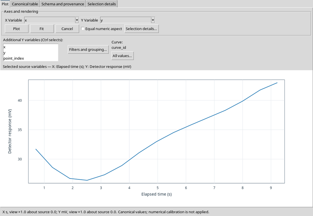
This makes it possible to distinguish the still-editable Interactive Document from the canonical scientific data already consolidated.
29. The Columns Actually Published
The canonical table shows X, Y, point identifiers, original raster coordinates and the three uncertainty columns.
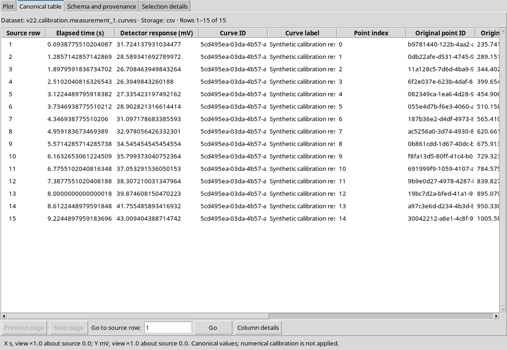
For physical_override the X standard uncertainty is 0.03 s and the Y one is 0.20 mV, with no XY covariance. For pixel_calibration the values change along the curve according to the transformation and the common factors. The point_id values, however, stay identical.
30. Metadata Schema and Provenance
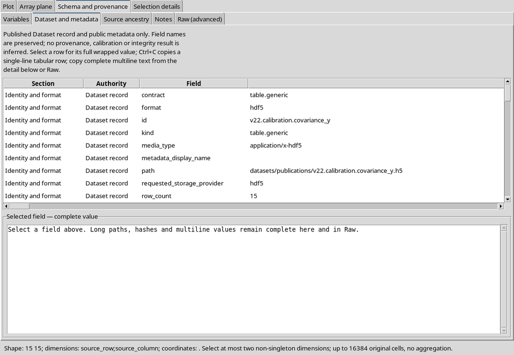
The Schema and provenance section contains the keys published by Curve Digitalizer.
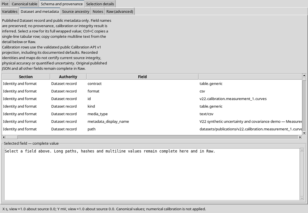
The uncertainty schema examined is version 2.
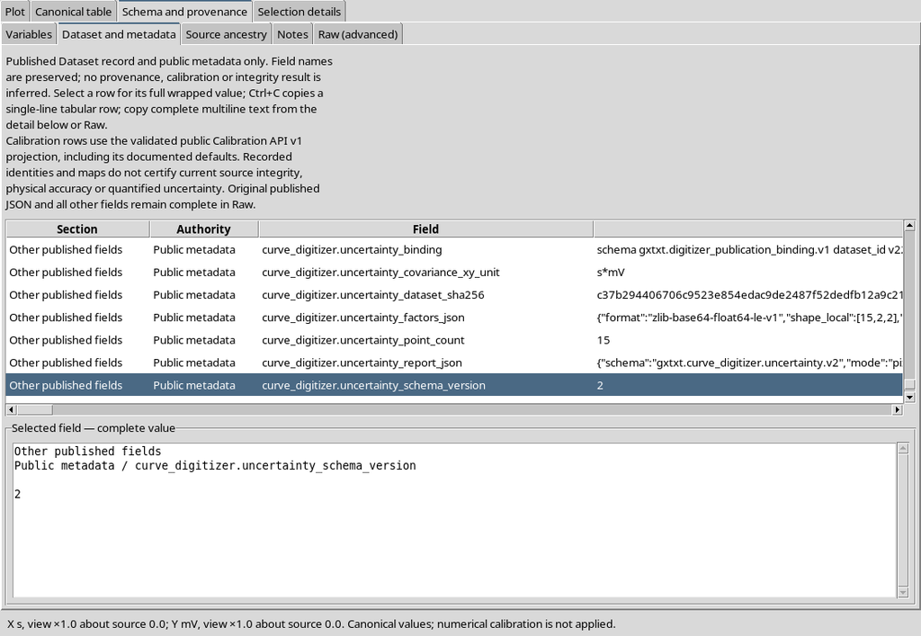
The metadata include the references to the source and to the canonical bytes, needed to verify that the declaration is linked to exactly the published Dataset.
31. Reading the JSON Report of the Declaration
The uncertainty report records mode, inputs, justification, units, calibration and a flag for the presence of shared factors.
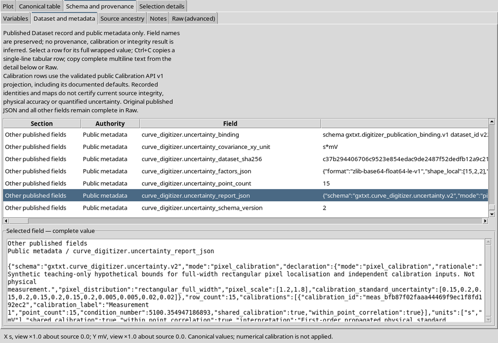
This is portable scientific information: another framework tool can read it without knowing the position of the fields in the graphic editor.
32. Compact Factors and Numerical Identity
The model keeps local and shared factors in compressed form, with a schema and a hash of the numerical bytes.
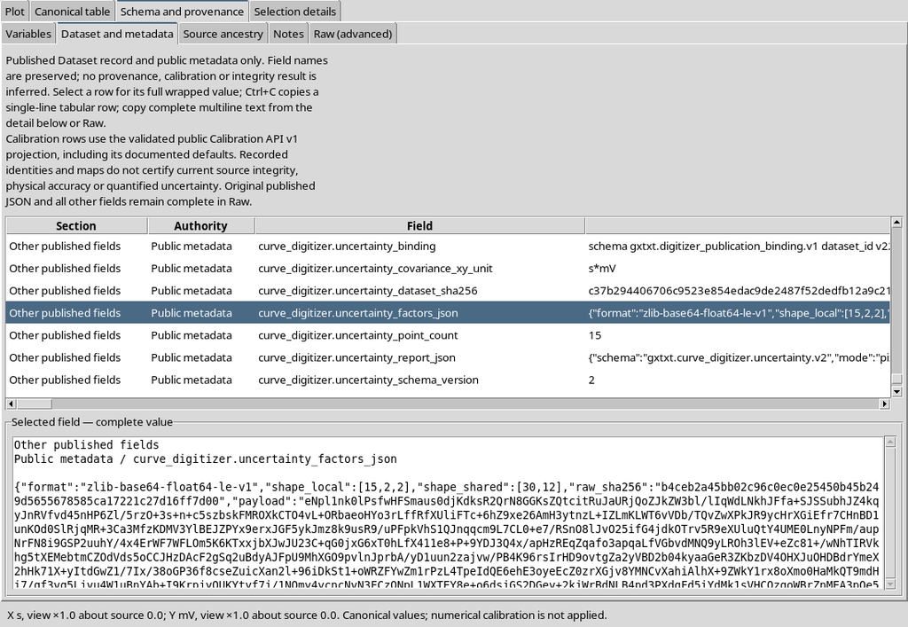
With 15 points and 12 common inputs, the shapes are 15 × 2 × 2 for the local factors and 30 × 12 for the shared ones. From these data the covariance can be rebuilt without wrongly treating all points as independent.
33. The CORE Review and the Numerical Source
Publishing with uncertainty enabled depends on the NUMERIC_API_v1 service and on the interpretation of the CORE Statistical Result Semantics. A preview computed locally in the GUI is not enough.
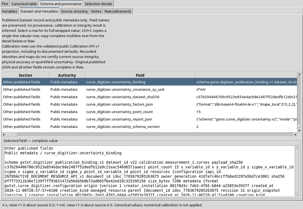
The SHA-256 of the published Dataset is kept together with the declaration.
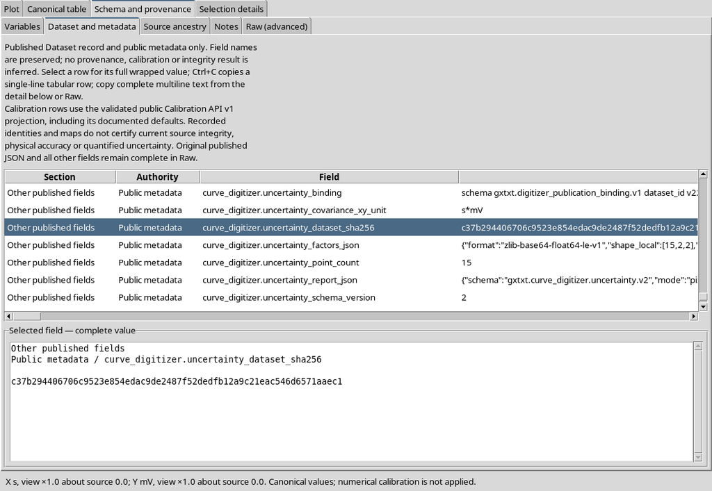
This identity protects the link between points, model and result: changing the canonical bytes afterwards would invalidate the review.
34. Publishing the Full Covariance of the Y Response
For this example, the public API authorized the publication of an HDF5 Dataset containing a full 15 × 15 matrix of the Y response.
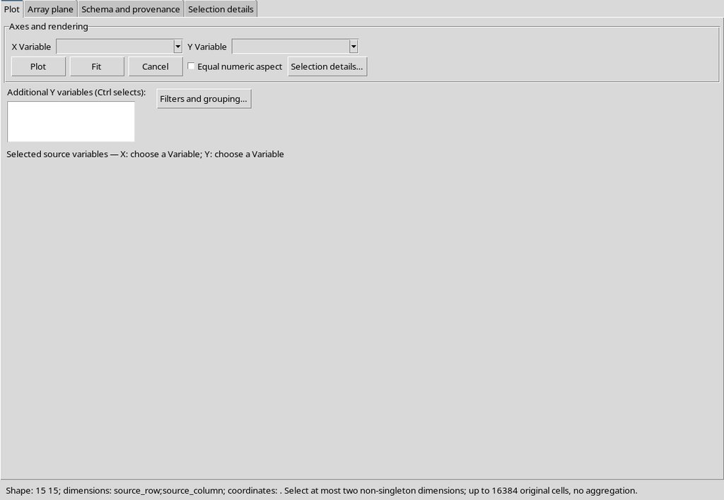
The matrix is a standalone output, distinct from the fifteen rows with the marginal sigmas. In the CORE Viewer it appears as a two-dimensional variable in the Array plane tab.
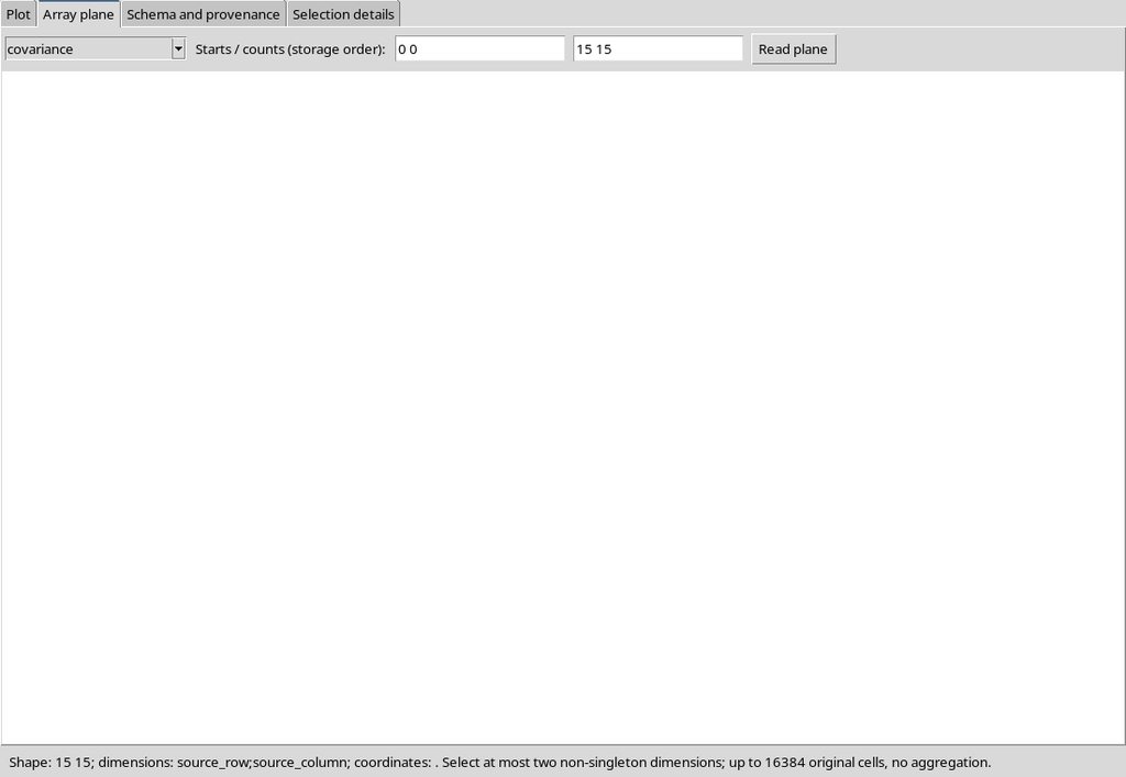
The metadata document the unit mV·mV, i.e. the covariance of the response in squared physical units.
35. Reading the Matrix and Checking the Correlations
With Read plane, the CORE Viewer displays the covariance matrix.
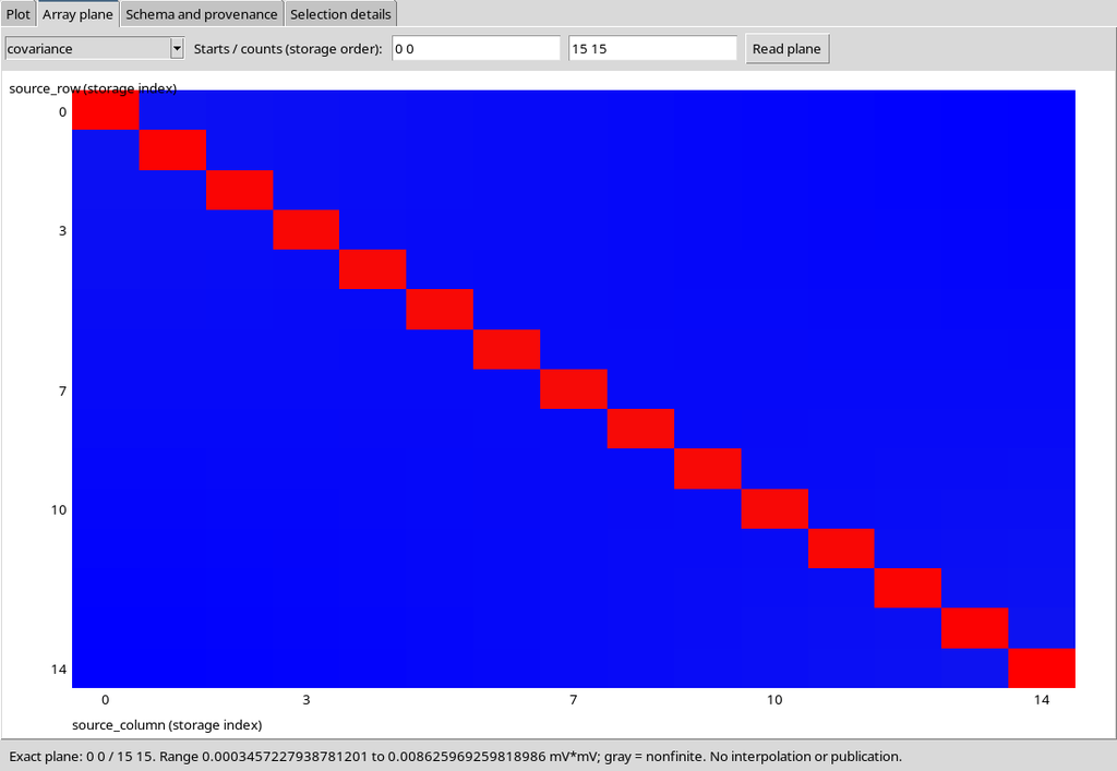
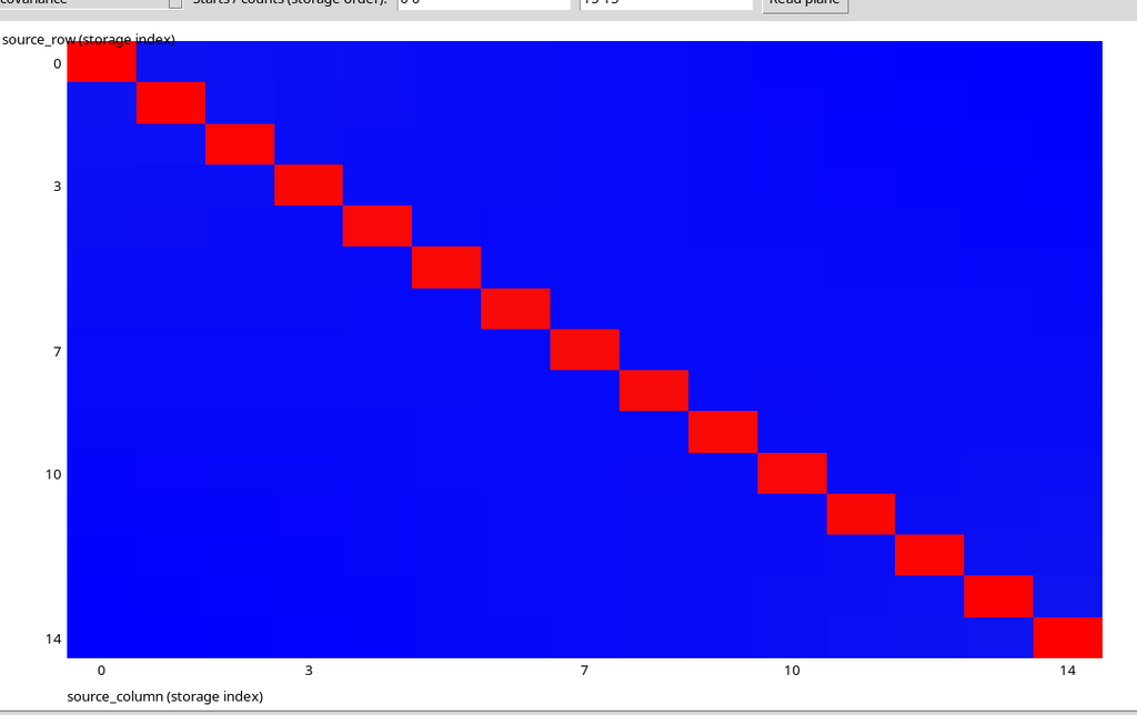
The off-diagonal components are not zero. The example was also checked by independently rebuilding the 225 elements from the published local and shared factors: the maximum absolute difference from the HDF5 matrix is about 5.2 × 10⁻¹⁸ mV², a numerical rounding residual.
This demonstrates the technical consistency of the results of this test, not the exactness of an instrumental measurement.
36. One Dataset for Each Meaning
The Dataset browser shows the source and the separate outputs:
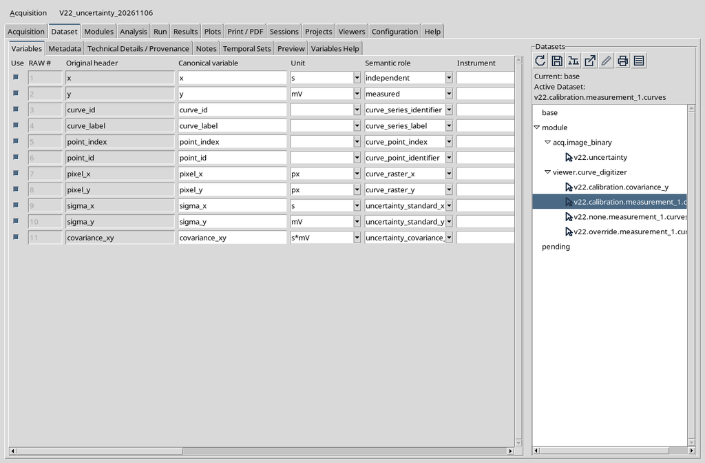
The none Dataset keeps only the points; physical_override contains the two declared sigmas; pixel_calibration contains the localization and calibration propagation; the covariance_y Dataset adds the full Y matrix.
A report already published is not rewritten automatically when the points are changed later in the Viewer.
37. Reading the Public APIs and Qualifying the Fit
Tcl example to run in the GX-TXT environment with an active Session. Replace the example Dataset identifier with the one actually published:
# Activate the public, versioned Curve Digitalizer uncertainty API.
::GX::modulePublicApiActivate viewer.curve_digitizer CURVE_DIGITIZER_UNCERTAINTY_API_v1

set dataset_id "example.published.curves"
if {![::GX::CurveDigitizerUncertainty::hasReport $dataset_id]} {
    error "A CORE-reviewed uncertainty report is required."
}

# Read the validated declaration and its original-row factor model.
set report [::GX::CurveDigitizerUncertainty::read $dataset_id]
set details [::GX::CurveDigitizerUncertainty::reportJson $dataset_id]
set factors [::GX::CurveDigitizerUncertainty::factorsJson $dataset_id]

# Inspect the authoritative CORE interpretation before using the model.
set reviewed [::GX::CurveDigitizerUncertainty::coreMeaning $dataset_id]
The same public API provides publishCovariance(datasetId, outputId, axis), to publish a full matrix when the CORE authorizes its interpretation. The operation generates a new canonical Dataset: it must be run deliberately with a free output identifier.
For this example the CORE judged the full_response_covariance / y_of_x plan admissible. This qualification concerns the response covariance for a possible GLS: the uncertainty of the X predictor is not included. It is not equivalent to a fit already performed and does not automatically authorize any ODR or GLS algorithm.
38. Scientific and Operating Limits
The declared uncertainties are standard uncertainties, conditional on the distributions and on the calibration model provided. They are not confidence intervals, nor an automatic estimate of accuracy.
The published contract sets limits of 4096 rows for propagation and 512 rows for materializing the full matrix. The single-axis model uses twelve shared inputs; a Y1/Y2 system uses fourteen. This guide exercises only the single-axis case.
When several calibrations are published with declared uncertainties, they must be treated as separate realizations until a validated model of the cross-correlations exists. Moreover, a physical scale bar is not automatically described by the uncertainties of the eight corners of a homography.
The Quality and Stroke width reports do not replace a physical declaration. In the Quality report the accuracy status stays not_assessed: a standard uncertainty declaration, even if propagated by the CORE, is not a verification of the accuracy of the instrument.
39. Recommended Verification Procedure
- Keep the original raster and check the calibration before acquiring the points.
- Publish without uncertainty when no justified model is available: do not invent sigmas.
- If you have metrological data, choose physical_override or pixel_calibration according to the real meaning of the inputs.
- Specify units, distribution, values and justification; do not leave the model implicit.
- Press Apply and save declaration and check that the review has been recorded.
- After any change to the points, the source or the calibration, re-examine the declaration before publishing.
- Check in the public metadata the uncertainty schema, the SHA of the Dataset and the outcome of the Numeric review.
- If correlations between points are needed, read the shared factors or publish a full covariance through the authorized public API.
- For fitting, use the CORE scientific plan and check which variables and correlations are actually included.
The conclusion is central: a numerically well-computed covariance is valid only with respect to explicit, justified metrological assumptions. GX-TXT can keep them, propagate them and make them verifiable; it cannot derive an instrumental precision from the appearance of the graph alone.