

Dataset Preview — Consulting Canonical Data and Point Traceability
The Canonical Data tab of the Dataset Preview lets you read the scientific coordinates published by the Curve Digitalizer and trace, for each point, the identity of the curve, of the calibration and of the position on the original raster. It is a consultation view: it does not modify the Dataset and does not reconstruct the data from the image.
To illustrate pagination we use a synthetic teaching raster of 1280 × 900 pixels. Three of the five traces were digitized with 22 points each, for a total of 66 canonical rows. The points include intermediate positions added along the synthetic traces through the Viewer: they do not represent experimental measurements, nor do they constitute an estimate of physical uncertainty.
1. Why Canonical Data Is Needed
A plot can show the correct curves, but it does not always allow all the points, their identities and their origin information to be distinguished. Canonical Data adds to the graphical representation a tabular reading of the values actually published.
It is useful for checking the numbers before carrying out subsequent analyses, distinguishing the various curves and recognizing the provenance of the points. The source remains the canonical Dataset of the Session.
2. The Calibration Before Publishing
The work starts from the Curve Digitalizer, with the X axis Elapsed time (s) from 0 to 10 and the Y axis Detector response (mV) from −20 to 80, on linear scales. Four calibration references BL, BR, TL and TR were accepted.
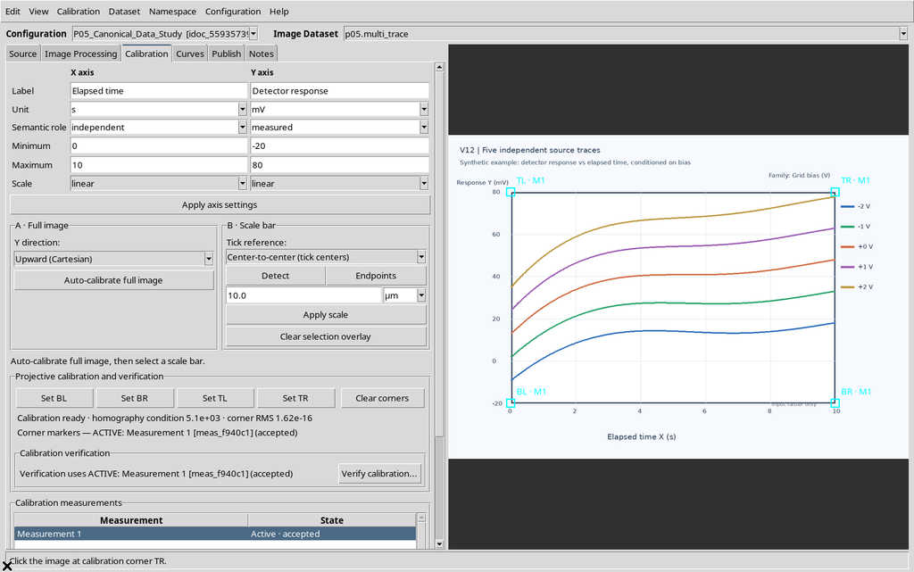
The calibration defines the transformation between pixel coordinates and scientific coordinates. Magnifying the table or the plot does not change this transformation.
3. Three Independent Curves to Exceed One Page
In the example Bias -2 V, Bias -1 V and Bias +0 V were created, each with 22 points. To obtain a sufficiently long exercise, intermediate positions were inserted on the synthetic drawing, without using an instrumental acquisition.
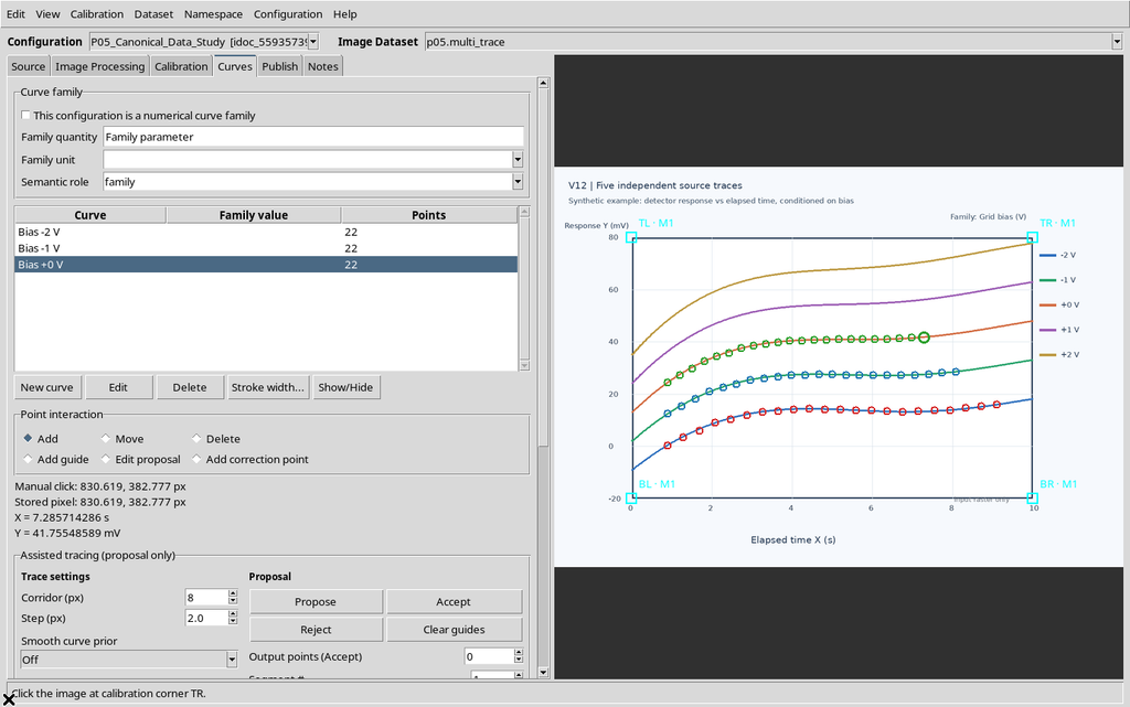
The two additional traces of the original raster are not part of the published curves. An image with five lines does not imply the presence of five numerical series.
4. Choosing the Numerical Output to Publish
In the Publish tab an accepted calibration and the separate mode were selected. The plan shows the numerical Dataset planned for that realization.
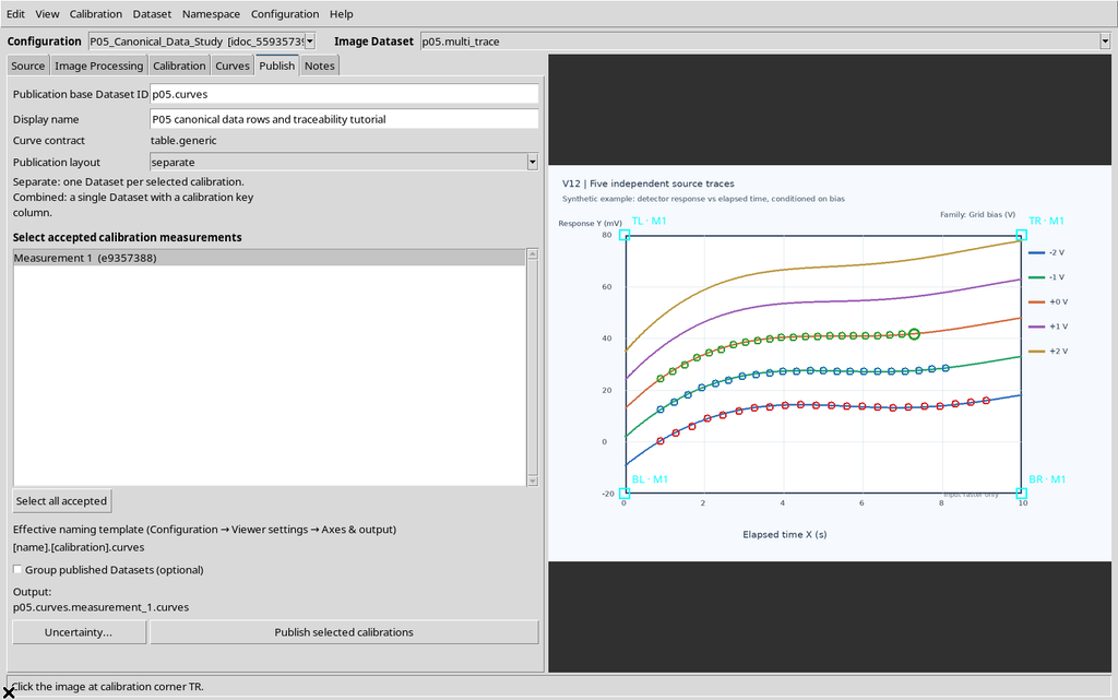
The identifier of the output Dataset must be distinct from the ID of the source image. The numerical publication keeps both references.
5. Confirming the Publication
Press Publish selected calibrations. In this case the Viewer confirms a successful publication, with one numerical Dataset, three curves and 66 scientific rows.
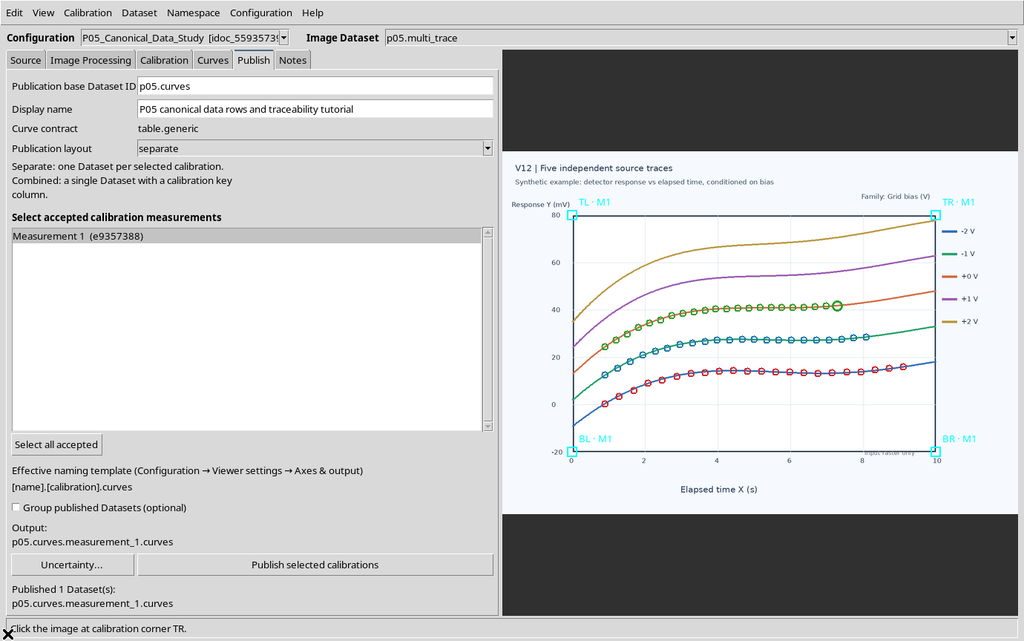
There is no need to repeat Publish to change the page, the display or the number of digits in the table.
6. Selecting the Dataset in the GX-TXT Browser
In the main window open Dataset → Preview. In the Datasets panel choose the numerical publication, not the previous Image Dataset.
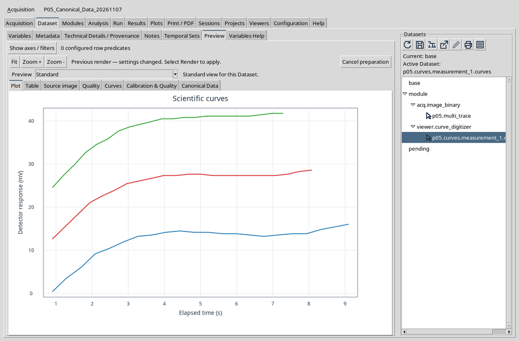
The Canonical Data tab appears when the Preview recognizes a compatible publication and the corresponding contribution is available.
7. The First Opening Does Not Read All the Rows
Select Canonical Data. Before the data are requested, the tables may be empty. The panel message indicates that the first page should be loaded.
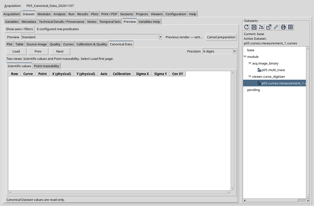
The initial emptiness is not equivalent to a Dataset without points: the user still has to request the page.
8. Load, Prev, Next and Precision
The top bar shows Load, Prev, Next and the Precision selector. The first three control access to the canonical pages; Precision changes the numerical format displayed.

In the example, after Load, the first page contains up to 50 rows. The CORE prepares the data through its own services, without a separate CSV reader in the Preview.
9. Loading the First Page with Load
Click Load. The first page of canonical values opens, with a message specifying the number of rows available and the state of the next page.
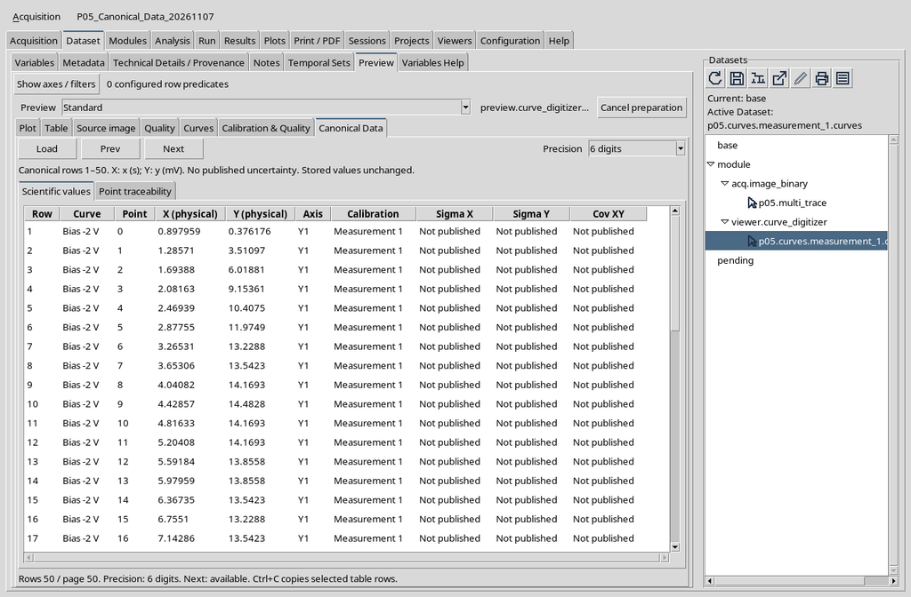
The example returns Canonical rows 1–50. The values are not recalculated while the table is being read.
10. The Scientific Values Columns
The Scientific values table contains Row, Curve, Point, X (physical), Y (physical), Axis, Calibration, Sigma X, Sigma Y and Cov XY.
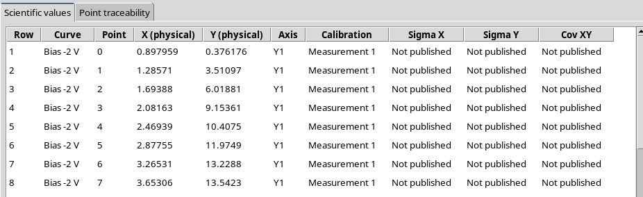
X and Y are the coordinates expressed in the published units; in the example, s and mV respectively. The other columns describe identity, ordering and any uncertainty fields available.
11. Row and Point Are Different Numberings
Row identifies the position of the row in the Dataset, starting from 1. Point represents the order of the point within the curve, starting from 0 in the example.
When a new curve begins, Point restarts from zero while Row continues to increase. Do not use either of these two numbers as a substitute for the persistent identifier of the point.
12. Switching from Scientific Values to Point Traceability
Select the Point traceability sub-tab. The values shown are linked to the same canonical rows, but the table exposes the technical references needed to reconstruct their provenance.
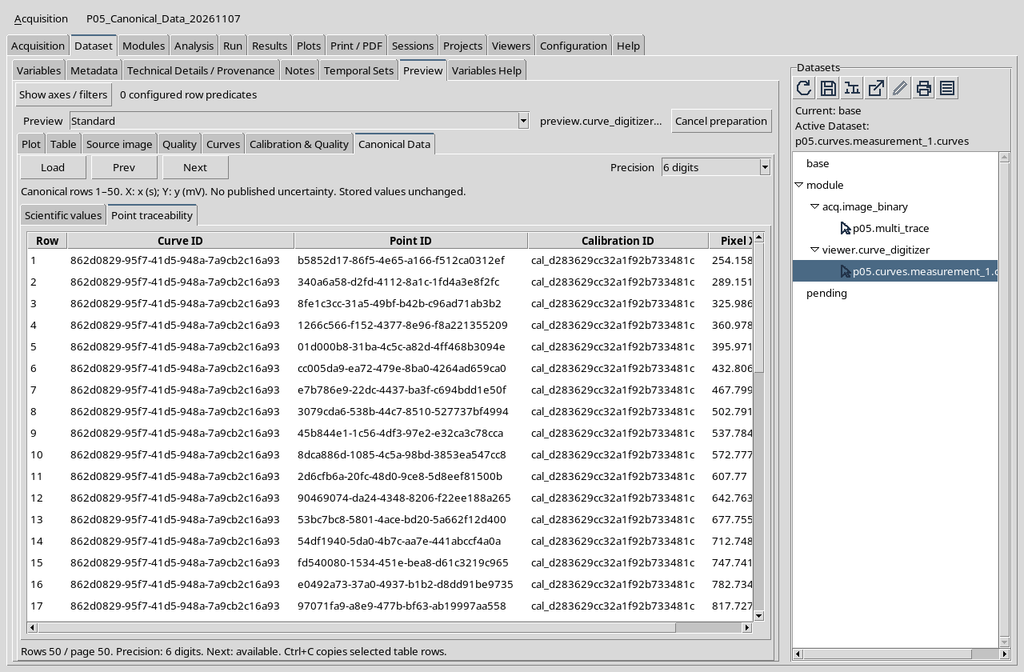
It is a change of view of the same Dataset: it does not create another independent scientific table and does not modify the calibration.
13. Curve ID, Point ID and Calibration ID
The Curve ID, Point ID and Calibration ID columns identify, respectively, the series, the individual point and the calibration used for the publication.
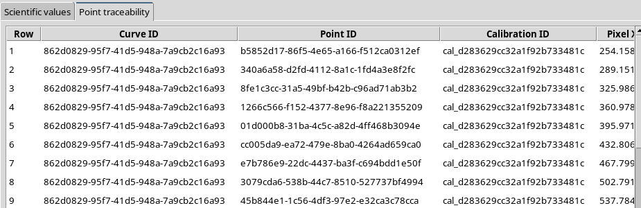
These identifiers must be treated as references, not as values to be converted into abscissas or ordinates. Any similarity between two readable names does not guarantee the identity of the objects.
14. Pixel X and Pixel Y Are Not the Physical Coordinates
The Pixel X and Pixel Y columns show the positions on the original raster. They must not be confused with X (physical) and Y (physical), obtained from the calibration transformation.
For example, a horizontal position measured in pixels is not automatically a time in seconds. The pixel coordinates serve above all to link each row to the source.
15. How to Interpret Traceability
Use the Row value to match, on the same page, a row of the Scientific values view with the corresponding row of Point traceability. The Point ID makes it possible to identify the point even when the curve name is not specific enough.
In this separate-mode publication, the calibration identity is unique for the three curves. A combined publication may require explicit differentiation between realizations: do not assume that all Datasets have the same schema.
16. The Second Page with Next
The initial view contains 50 rows. Press Next to consult the remaining rows, from 51 to 66.
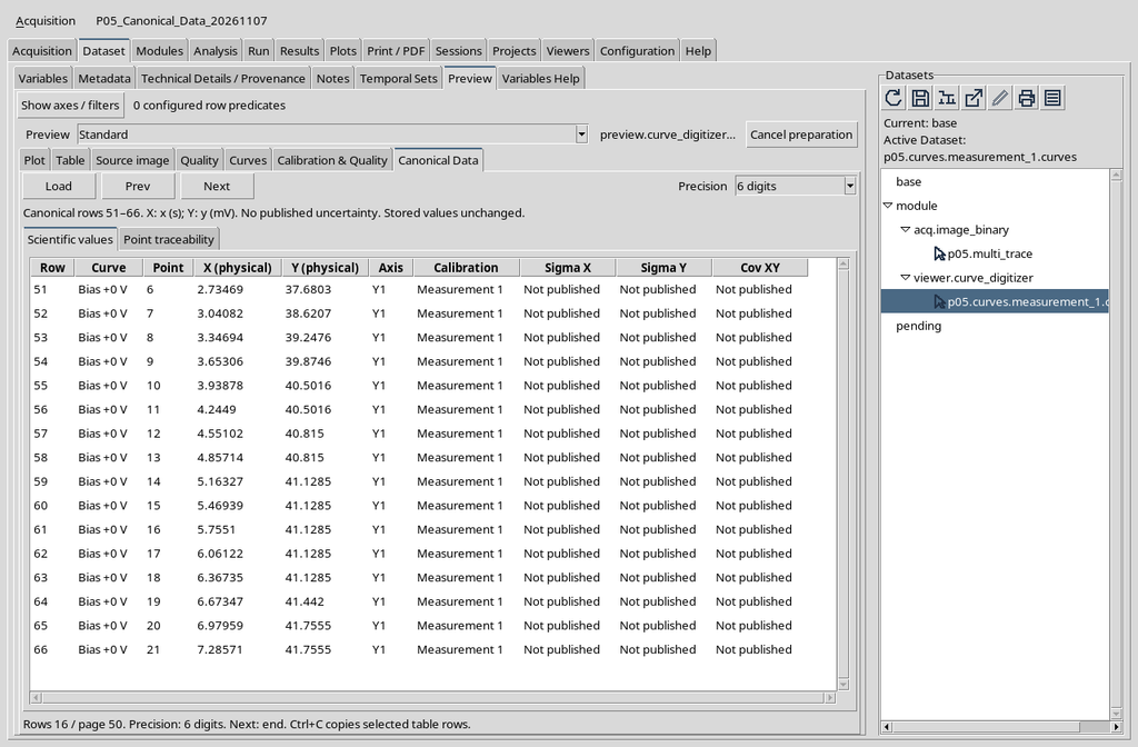
The next page does not start from 1: the row number keeps the original position in the Dataset.
17. Point Traceability on the Second Page
On the 51–66 page too you can switch to Point traceability to see the identities and raster coordinates of the remaining points.
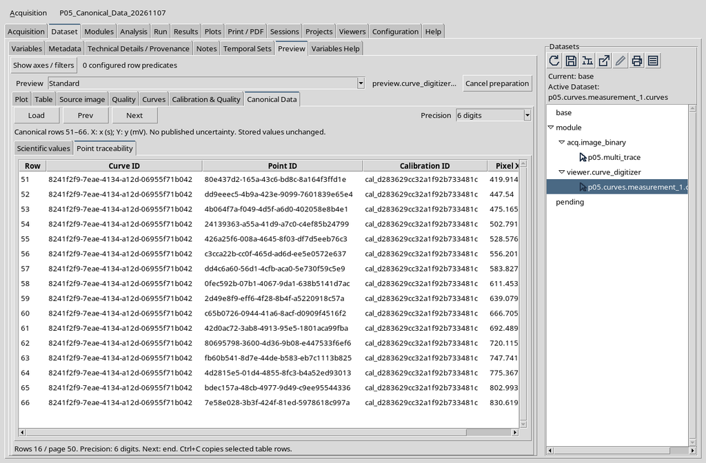
Switching from one sub-tab to the other must not alter the selected page: the same rows are consulted in two different representations.
18. What Happens When Pressing Next on the Last Page
When there are no further rows, the status message indicates Next: end. The Next command may remain visually clickable, but in the installation shown a further click does not change the page.

Check the row number and the end-of-page message, not just the appearance of the button.
19. Going Back with Prev
Press Prev to return to the first 50 rows. The numerical values and identifiers of the page already read reappear without a new publication.
On the first page, pressing Prev again does not produce a page with negative numbers. Navigation remains within the limits of the current Dataset.
The Prev command lets you return to the page with Canonical rows 1–50. The recovered screen is identical to that of the first Point traceability page already illustrated: there is no need to duplicate it to show the return.
To check the result, verify the row range indicated by the panel and the correspondence between Row, Curve ID, Point ID and raster coordinates. Changing page does not modify the persistent identifiers or create a new Dataset.
20. Load Returns to the First Page
The Load entry requests the first canonical page. It serves both at the first opening and when you want to restart the consultation from the beginning.
It is not equivalent to Publish. Reading can benefit from a CORE cache, while the scientific identity of the data and the number of rows remain those registered.
21. The Three Precision Options
The Precision selector offers 6 digits, 10 digits and Full precision. The options concern the way in which numbers already present in the Dataset are printed.
The choice does not increase the accuracy of the measurement, does not introduce new significant decimals into the instrument that generated the data and does not modify the stored canonical values.
22. The 6 Digits Format
On opening, 6 digits is used. In the case illustrated the first X coordinate is shown as 0.897959, with a limited number of digits.
This format is useful for quickly reading many rows. The displayed rounding does not erase any additional digits kept in the Dataset.
23. The 10 Digits Format
Open Precision and select 10 digits. The same first X is displayed as 0.8979591837: the digits shown change, not the physical position of the point.
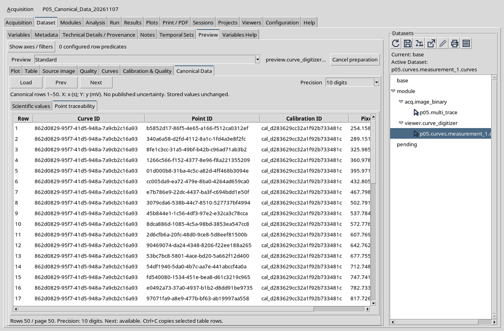
It is a compromise between readability and reproduction of the available digits.
24. The Full Precision Format
Select Full precision to show the full-precision numerical representation available in this view. In the case illustrated the first X coordinate is 0.89795918367347027.
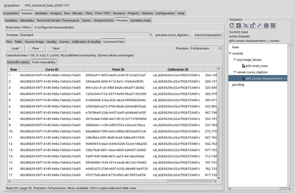
The value may appear with more digits than are useful for a real experiment. Precision of the numerical representation and measurement uncertainty are different properties.
25. The Digits Shown Do Not Change the Original Value
The Full precision choice avoids part of the display rounding, but it is not a declaration of experimental accuracy. Text representations of floating-point numbers may differ in form while expressing the same numerical value.
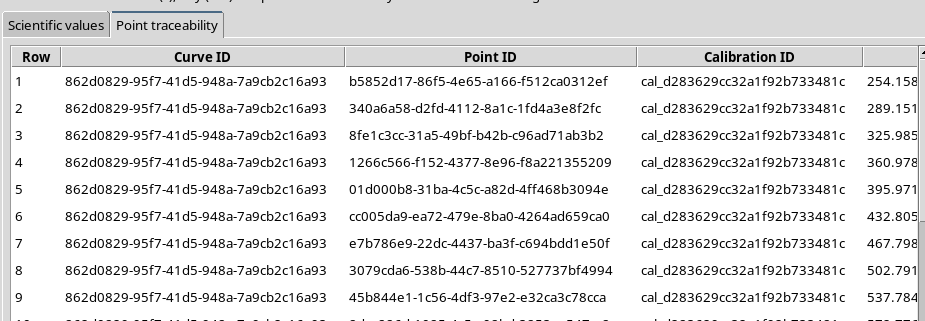
For a rigorous check, use the Dataset APIs and traceability, not the simple count of decimals visible in a cell.
26. Returning to the 6 Digits Display
After examining the values at full precision, select 6 digits again. The table returns to the initial format.
The same principle applies to the pixel coordinates in the Point traceability sub-tab.
After selecting 6 digits, the same page returns to the abbreviated representation, without losing any numerical digits stored in the Dataset. The screen is identical to a view already presented and is therefore replaced here by this explanation.
A correct comparison between 6 digits, 10 digits and Full precision must concern the same row and the same point identifier. The textual differences depend on the display format, not on a new transformation or an increase in experimental accuracy.
27. Precision and Pagination Are Independent
Precision can also be changed after reaching the second page. The format selection acts on the rows currently displayed, without necessarily returning to the beginning.
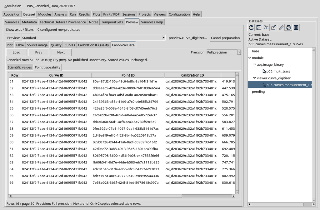
When comparing two screenshots, therefore, check both the active page and the selected Precision option.
28. Sigma X, Sigma Y and Cov XY
The scientific table also contains the Sigma X, Sigma Y and Cov XY columns. In this example they show Not published, because the publication does not include a numerical declaration of physical uncertainty for the points.
An unpublished field must not be read as zero. When correctly declared uncertainties exist, their units must be consistent with the scientific axes.
29. Comparison with the Curves Tab and Plot Dataset v4
Switching to the Curves tab of the same Preview and pressing Load curves gives the native plot of the three series, now with 22 points each.
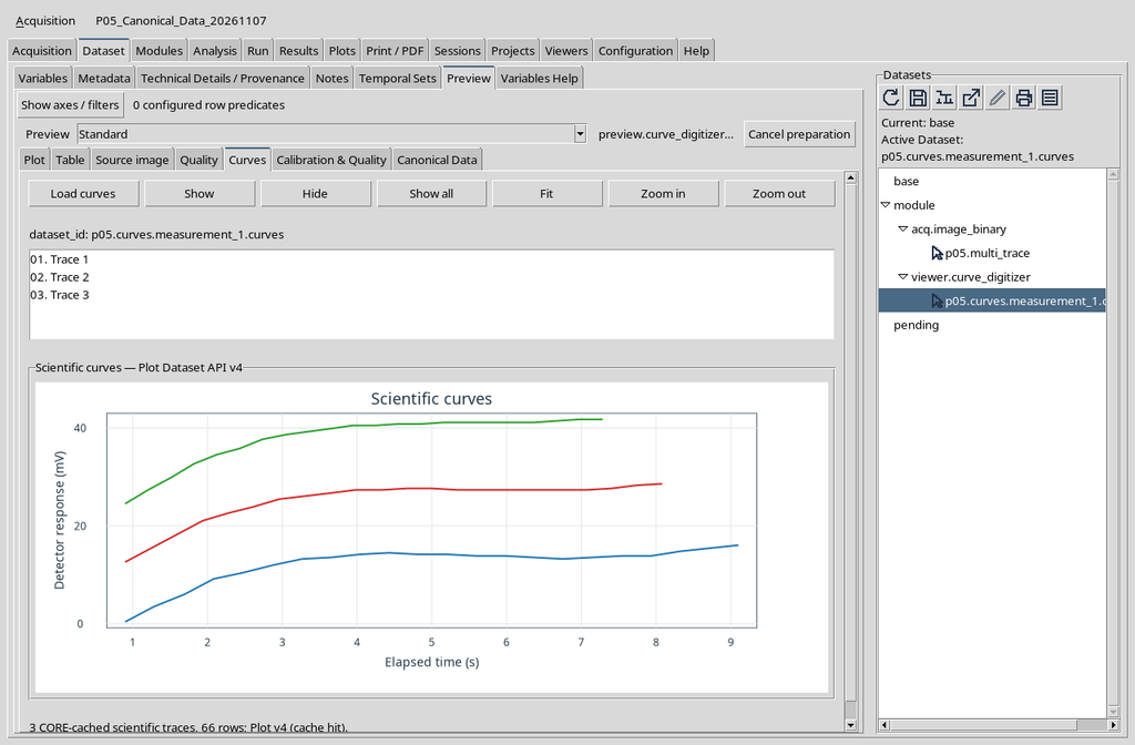
The table and the plot are not two publications: they represent the same Dataset with different tools.
30. Hiding a Curve in the Plot
With the first trace selected, press Hide in the Curves tab. The first line disappears from the plot, while the others remain visible.
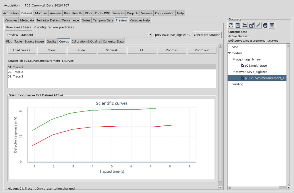
This command modifies the presentation. It must not be confused with deleting the curve within the Viewer’s editable document.
31. Returning to Canonical Data After Hide
After hiding a line, return to Canonical Data. The rows of the hidden curve are still present in the table, with the same values and identifiers.
This is an important check: a visibility filter must not modify the Dataset on which subsequent analyses will be carried out.
To carry out the check, return to the Canonical Data tab, press Load if the page is not already available and check that the rows of the hidden curve can still be consulted. The X (physical) and Y (physical) values and the identifiers must correspond to those read before Hide.
The same traceability table has already been illustrated above: the essential point is not to reproduce another image, but to distinguish the graphical Hide filter from deleting data. The visibility of a curve does not determine the content of the canonical Dataset.
32. Restoring All Curves with Show All
To return to the complete plot, press Show all in the Curves tab. The renderer presents the three series again using the points already published.
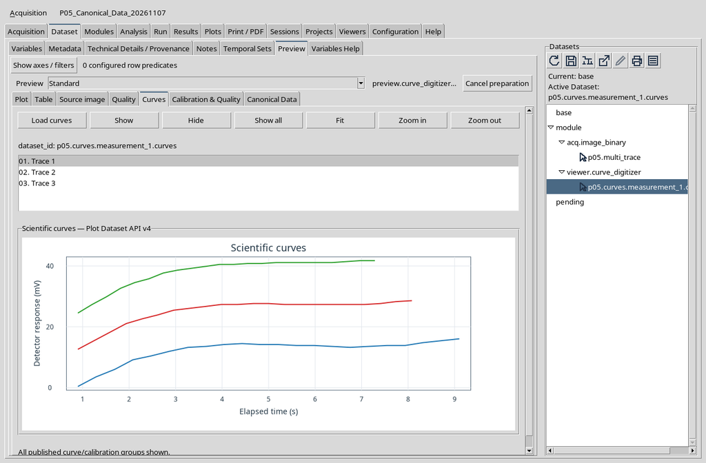
Even when switching from Plot to Canonical Data and back, the relationship between image, points and canonical rows remains the same.
33. Cross-Checks on the Two Pages
In the case illustrated, reading the two pages returned 50 + 16 = 66 rows. The 66 rows were compared with the CORE public pagination service, checking both the scientific coordinates and the traceability identifiers.
The 6 digits, 10 digits and Full precision formats were also checked: the format conversion does not alter the stored numerical content.
34. Identifiers Allow Better Checks Than Colours
The series shown in blue, red or green may change colour in another plot. The Curve ID and Point ID identifiers, instead, make it possible to recognize the provenance of the point without depending on the graphical palette.
When a scientific analysis needs to be documented, keep the link between numerical Dataset, variables, calibration and original raster. Do not reconstruct the identifiers from colours or display names.
35. Summary of the Consultation Flow
The operating flow is Dataset → Preview → select the numerical Dataset → Canonical Data → Load. Consult Scientific values, switch to Point traceability, use Next/Prev for the pages and Precision for the number format.
In our exercise the Dataset contains three synthetic curves for 66 points, keeps the relationship between physical coordinates and original pixels and remains unchanged after reading the pages, changing precision and the Show/Hide operations in the Plot. The canonical content and its provenance are distinct from the form in which they are presented.