

GX-TXT Python Script Workspace: building a multi-file Project and exploring it with the debugger
This tutorial shows how to create a real Python Project with a main file and a package of auxiliary functions, save it as a single revision, follow the execution in the native debugger and read Call Stack, Locals and Globals. The processing uses synthetic data: no real instrument or Dataset is needed.
1. Scientific and teaching aim
We will carry out a simple multiplicative calibration with synthetic readings [1.0, 4.0, 9.0] and factor 2.0. The support function returns [2.0, 8.0, 18.0]; the expected final result is 28.0. The example serves to understand the distinction between main source, helper file, Project Registry, Debug Job and program output. It does not compute uncertainties and does not publish Datasets.
2. What a Python Project is in GX-TXT
A single Script contains a single source; a Project gathers several Python files with a common identity, entrypoint and revision. The helper files are imported by the main file following normal Python syntax, but are kept as part of a snapshot of the Project. There is no need to open the Script Library: all the operations described are available directly in Python Script Workspace.
3. Creating the Project from the original window
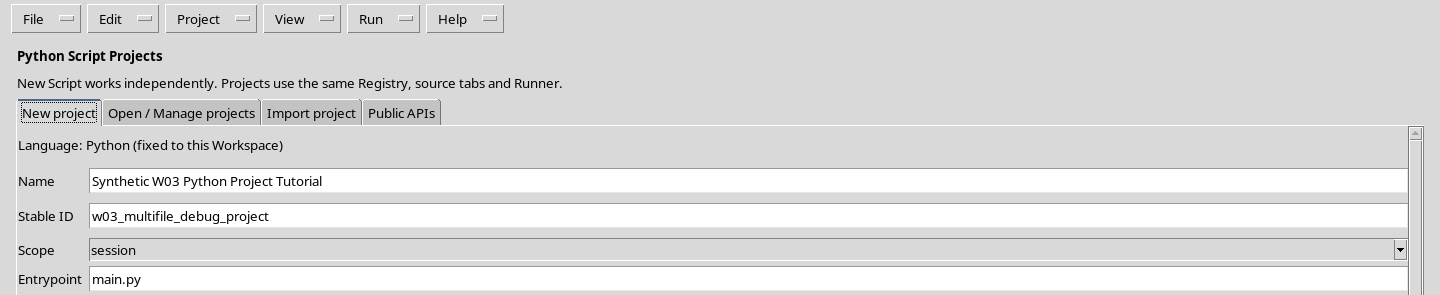
Open your own Session, start Python Script Workspace, then choose Project → New Project…. In the form set a descriptive name, a Stable ID such as w03_multifile_debug_project, Scope to session and Entrypoint to main.py. Press Create project. The Session scope keeps the work together in the current scientific context.
4. The structure of the three files
The structure to obtain in the Project is:
main.py
helpers/
    __init__.py
    numeric.py
main.py is the entrypoint; helpers/numeric.py contains the computation; helpers/__init__.py identifies the package. The paths are relative to the Project. They must not be replaced with absolute paths of the computer.
5. Writing main.py
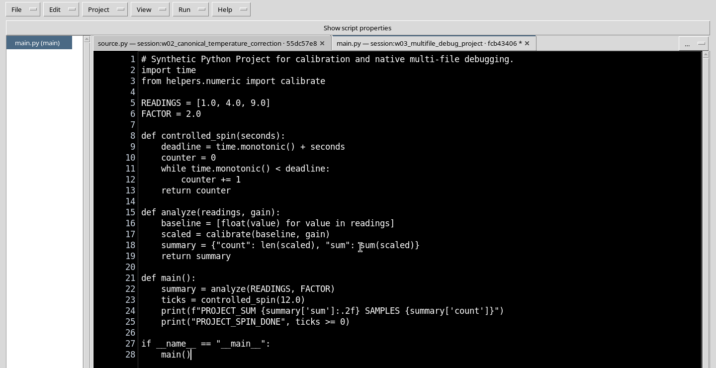
In the central pane edit main.py. The example imports calibrate from the helper file, defines three artificial readings, calls analyze and prints the total. The function controlled_spin adds a time-limited loop to observe the Pause command: it is a debugger demonstration, not an efficient model of waiting in scientific programs.
6. Adding a helper file
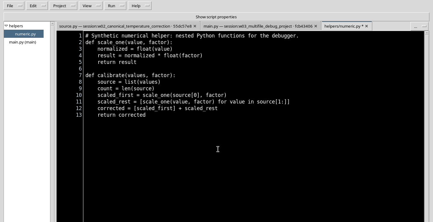
Choose Project → New file…. Enter the relative path helpers/numeric.py, then confirm with Apply. The editor opens the new file in a separate tab. Write the two functions calibrate and scale_one; the latter will be reached using Step Into.
7. Adding helpers/__init__.py
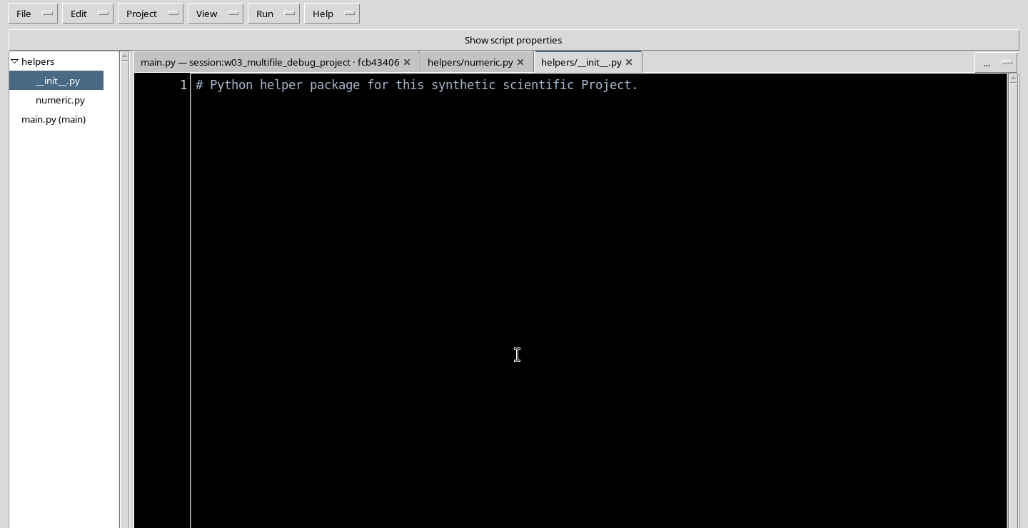
Repeat Project → New file… with helpers/__init__.py. In this example a comment describing the package is enough. Do not create a separate directory externally: the GUI command registers the file and includes it in the Project.
8. The complete code of the three files
The following program corresponds to the Project used in the exercise. All comments in the code are in English.
main.py
# Synthetic Python Project for calibration and native multi-file debugging.
import time
from helpers.numeric import calibrate

READINGS = [1.0, 4.0, 9.0]
FACTOR = 2.0

def controlled_spin(seconds):
    deadline = time.monotonic() + seconds
    counter = 0
    while time.monotonic() < deadline:
        counter += 1
    return counter

def analyze(readings, gain):
    baseline = [float(value) for value in readings]
    scaled = calibrate(baseline, gain)
    summary = {"count": len(scaled), "sum": sum(scaled)}
    return summary

def main():
    summary = analyze(READINGS, FACTOR)
    ticks = controlled_spin(12.0)
    print(f"PROJECT_SUM {summary['sum']:.2f} SAMPLES {summary['count']}")
    print("PROJECT_SPIN_DONE", ticks >= 0)

if __name__ == "__main__":
    main()
helpers/numeric.py
# Synthetic numerical helper: nested Python functions for the debugger.
def scale_one(value, factor):
    normalized = float(value)
    result = normalized * float(factor)
    return result

def calibrate(values, factor):
    source = list(values)
    count = len(source)
    scaled_first = scale_one(source[0], factor)
    scaled_rest = [scale_one(value, factor) for value in source[1:]]
    corrected = [scaled_first] + scaled_rest
    return corrected
helpers/__init__.py
# Python helper package for this synthetic scientific Project.9. Saving consistently with Save All
Use File → Save All when the three buffers are ready. GX-TXT registers a consistent revision of the whole Project, with identification of the files, entrypoint and content fingerprints. The modification stars on the tabs must disappear. Saving does not imply running the code; for scientific reproducibility the Job must always refer to the snapshot actually saved.
10. How importing the helpers works
The line from helpers.numeric import calibrate tells the managed Python to import calibrate from the Project package. The function calibrate calls scale_one, which turns each value into a float and multiplies it by the factor. analyze sums the results. This is normal Python; there is no need to invoke internal GX-TXT APIs to find the Project files. The runtime instead checks that the multi-file snapshot and the source names are allowed.
11. Preparing a breakpoint in the helper file
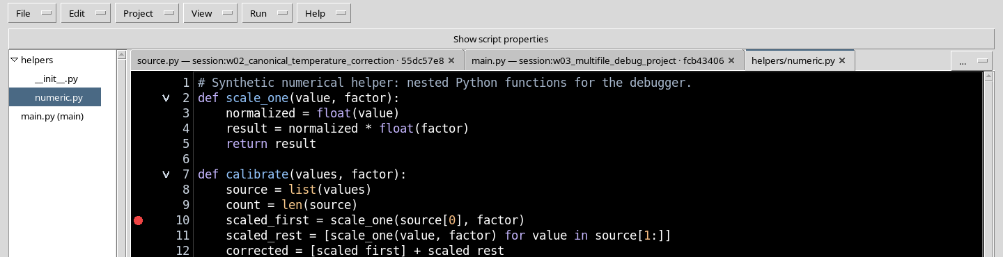
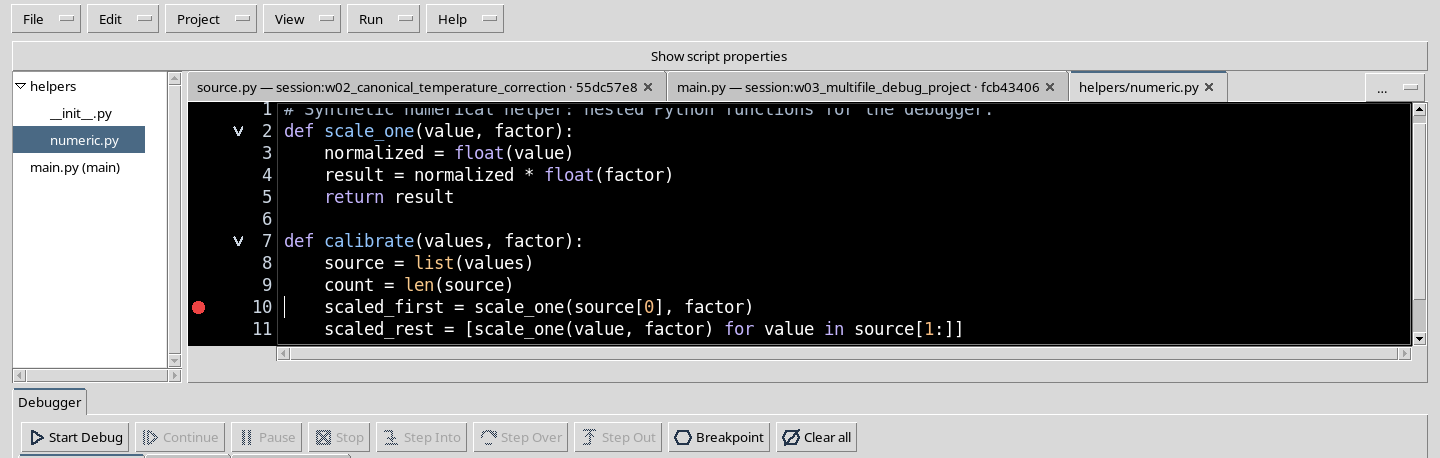
Open helpers/numeric.py from the Project structure. Move the cursor to line 10, scaled_first = scale_one(source[0], factor), and press F9. An indicator in the margin identifies the stopping point. A breakpoint is associated with the file and the line, not simply with number 10 of the entrypoint.
12. What changes when you use the debugger
A normal Run Job runs the program to completion or to an error; the Debugger controls a managed Job during its execution and can suspend it at defined points. The debugger buttons are operations on the actual Job, not simple animations in the editor. When a Debug Job is active, the code being run remains an immutable snapshot.
13. Opening Debug Session script…
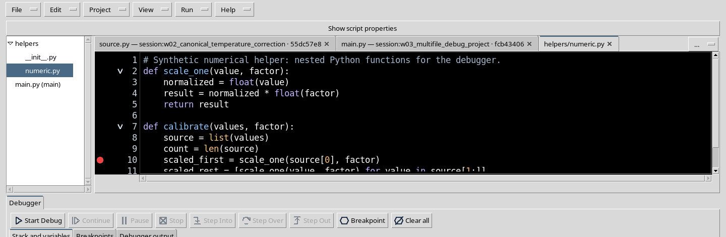
In the Run menu, choose Debug Session script…. The lower panel shows Start Debug, Continue, Pause, Stop, Step Into, Step Over and Step Out. Open only the Stack and variables sections needed for the explanation; for ordinary work it is preferable to keep superfluous panels closed.
14. Starting the debug Job and recognising the first pause
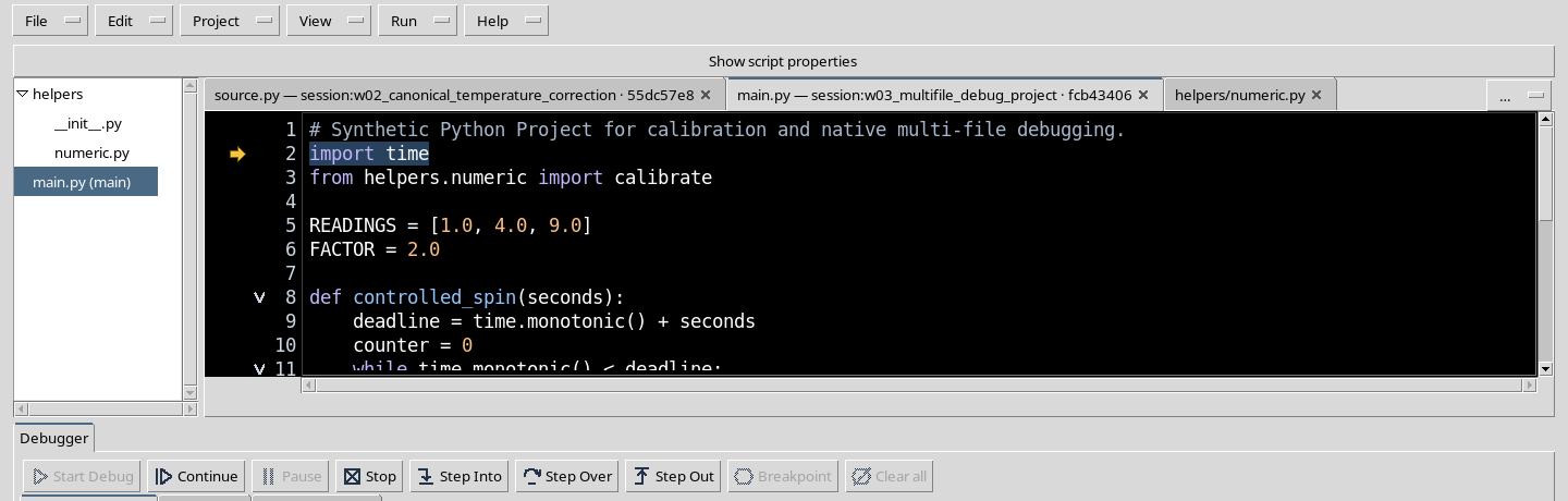
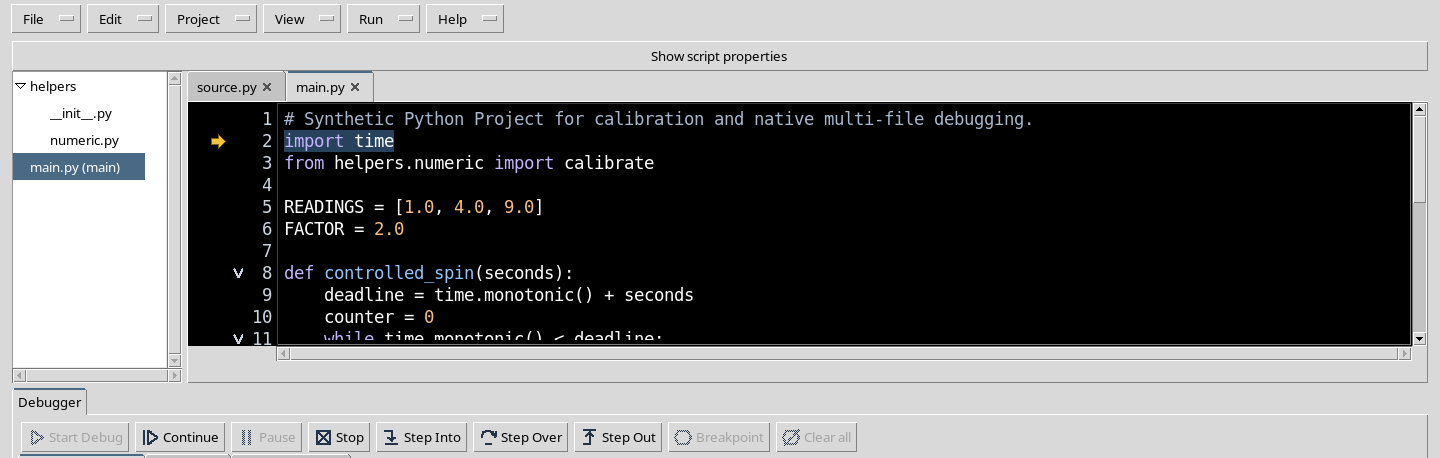
Press Start Debug. The runtime creates a managed Python Job and, before proceeding in the code, exposes the initial pause. The PAUSED state and the execution arrow indicate the next statement. In this state you can already observe the controls, but the most interesting local values will appear when you enter the calibration function.
15. Continue up to the calibrate call
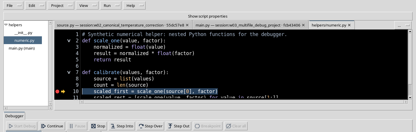
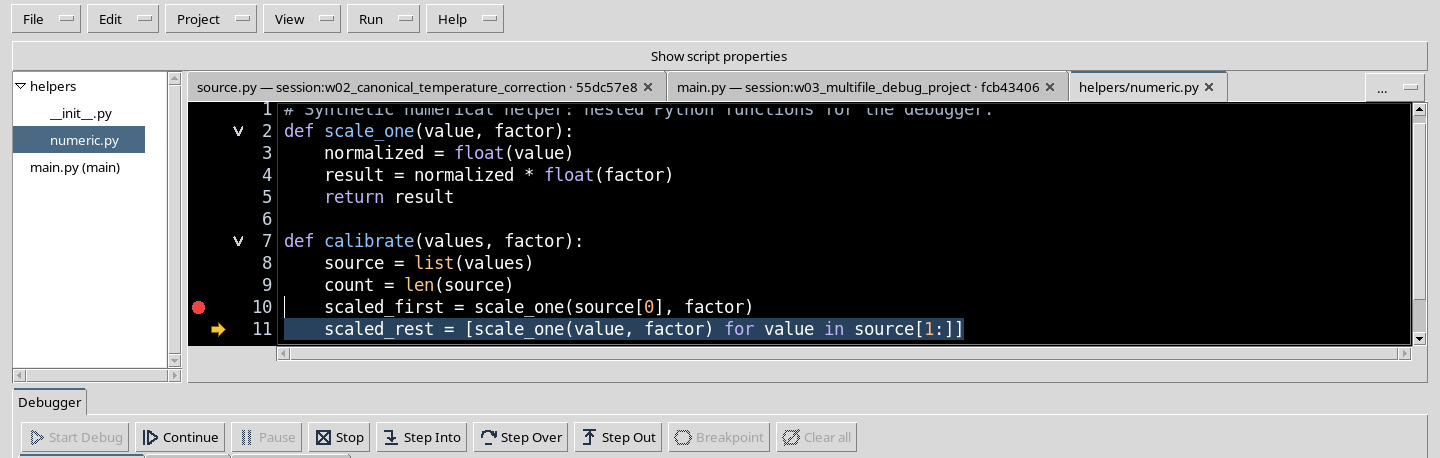
Press Continue. Execution reaches the breakpoint in the function calibrate, line 10 of helpers/numeric.py, before invoking scale_one. The breakpoint indicator and the execution arrow are distinct. Here you can read the input list of the function and the factor, while the subsequent assignments have not yet taken place.
16. Selecting the calling frame
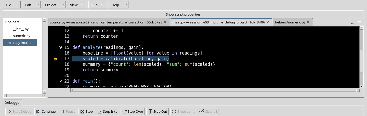
In the Call Stack, choose the analyze frame. The visible source switches to main.py, while the interpreter actually remains stopped in the calibrate frame. Selecting the frame is not the same as Continue and does not move the execution point; it lets you examine the state of a caller.
17. Reading the order of calls
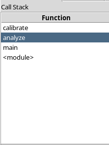
The visible sequence includes calibrate, analyze, main and the module frame. The top of the stack corresponds to the function in which the suspension occurred; below are the callers. The line number shown next to a frame identifies its source position, while the yellow arrow is reserved for the actual execution point.
18. Interpreting Locals and Globals
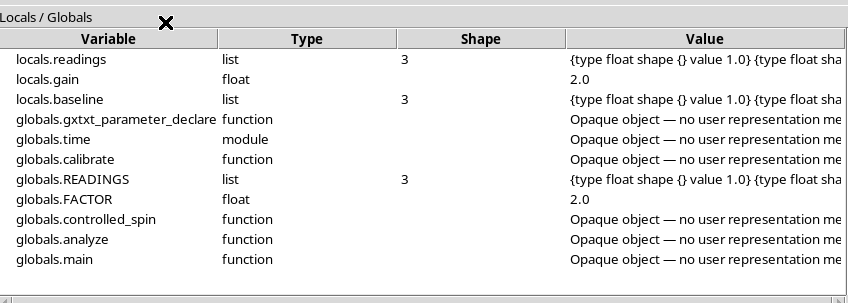
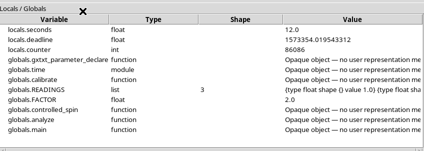
The Locals / Globals panel exposes names, types, shapes and values within display limits. In the calibrate frame, factor is 2.0, source has three values, count is 3; functions and modules are shown as opaque objects. When you switch to the analyze frame, the observable local values change. A variable not yet assigned must not be interpreted as already computed.
19. Step Into: entering the nested function
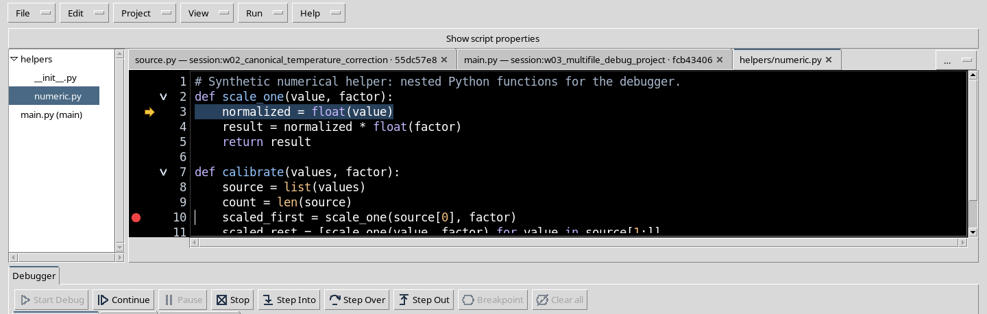
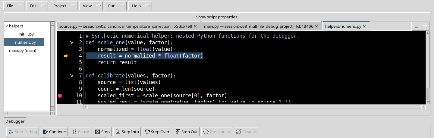
Return to the top frame calibrate and press Step Into. In this program you actually enter the function scale_one, stopping at line 3 before the statement normalized = float(value). It is the appropriate command when you want to inspect how a helper works instead of treating it as a single operation.
20. Step Over: running the current line
Press Step Over to run the current assignment without entering a new call. The next statement observed is line 4 of scale_one, result = normalized * float(factor). Debugging stays inside the same function and lets you observe how the local values change.
21. Step Out: returning to the calling function
Press Step Out. Execution completes scale_one and returns to calibrate, at line 11, where the transformation of the other elements is prepared. The debugger does not remove any frame: it displays the natural return of the Python call and the update of the stack.
22. Completing the first Debug Job
When you press Continue, the program completes the calibration, runs the limited loop and writes:
PROJECT_SUM 28.00 SAMPLES 3
PROJECT_SPIN_DONE True
The Job ends with state COMPLETED, exit code 0 and an empty stderr stream. The result mathematically confirms the sum 2 + 8 + 18 = 28. The code did not publish a canonical Dataset: this is text output. A Pause command accepted during a running Job does not, by itself, guarantee that the next observed state is PAUSED.
23. Preparing the asynchronous Pause demonstration
To observe an actual Pause, end and close the Debugger, reopen the Project if necessary, remove the previous breakpoint from the helper function and place F9 on line 24 of main.py, after the controlled_spin loop. The new breakpoint will remain to be reached; the loop uses a limit of twelve seconds only to make the RUNNING state visible. Start a new Start Debug, get past the initial pause and press Continue.
24. Pause during RUNNING: observing the actual result
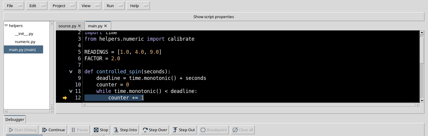
When the Debugger reports RUNNING, press Pause. In this test the request actually led to PAUSED in the function controlled_spin, at line 12. The arrow points to the statement counter += 1. The example shows that the asynchronous behaviour depends on the adapter and on the execution situation: always check the real final state instead of relying on the click of the button.
25. Locals during Pause and the difference between Stop and Completed
During this pause, Locals shows seconds = 12.0, deadline and counter with the values observed from the running Python. To interrupt the demonstration use Stop: the terminal state of this second Debug Job is CANCELLED, not COMPLETED. It is correct to distinguish the first Job, completed with the total 28, from the second execution, voluntarily interrupted.
26. Closing the debugger, reopening the Project and keeping the work
Close the debugger panel when the Job is terminal. If the editor does not allow you to insert or remove a breakpoint even though there is no longer an active Job, save the work and carry out the normal sequence File → Close, reopen Python Script Workspace and choose Project → Open Project…: the saved Project reappears with entrypoint and contents unchanged. This procedure was verified with the normal GUI path. Then keep the optional panels closed to give space back to the code. The Project remains in the Session; the Script Library is not needed, no instruments have been modified and no Dataset has been created.