GX-TXT Python Script Workspace: formatting Markdown notes and managing PNG images
The notes associated with a Python file can be formatted and enriched with images without running the program. This guide shows the commands actually available in the Notes editor: Note format, Note images, Resources, Properties, Save and Publish New. The example includes a small plot of synthetic measurements: it is a documentation image, not a numeric Dataset generated by a Job.
1. Documenting the source without changing the program
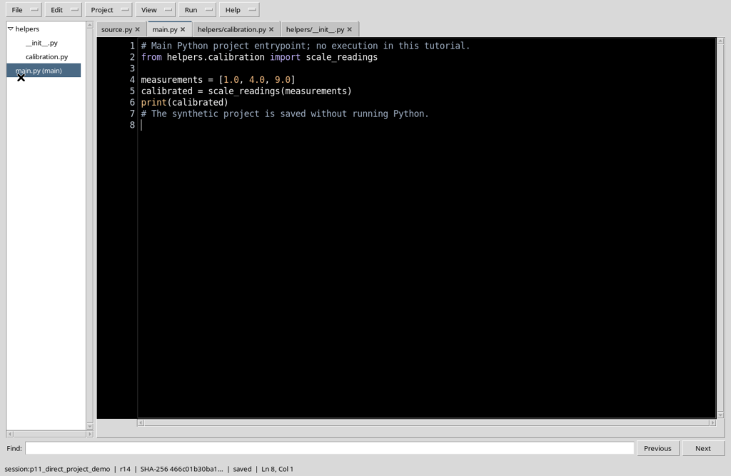
In Python Script Workspace, each file of a Project can have a separate Markdown note. The Notes tab is used to explain assumptions, inputs, expected result, limits and illustrative figures. Editing this note does not change the statements of the main.py file and does not start the Python interpreter. Documentation revisions and code content are therefore two different things.
2. Opening an existing note
Open a Project with an already saved Python file and select main.py. Choose Edit → Edit Notes. In the example the note already contains headings, a list and references to the helpers/calibration.py module. To work with persistent resources you need a valid Session and the ability to save the associated document. Without that context you can read the note, but you must not assume that images can be registered.
3. The commands of the Note format menu
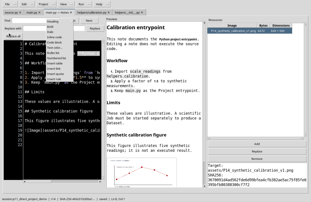
When the Notes tab is active, the Edit → Note format menu offers Heading (with Heading 1, 2 and 3), Bold, Italic, Inline code, Code block, Text color, Bullet list, Numbered list, Insert table, Insert link, Insert quote and Insert rule. They are commands for inserting or transforming Markdown text, not functions for editing Python code.
4. Applying Bold to a selection
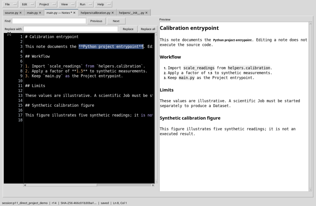
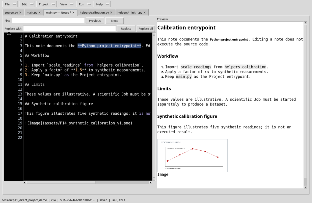
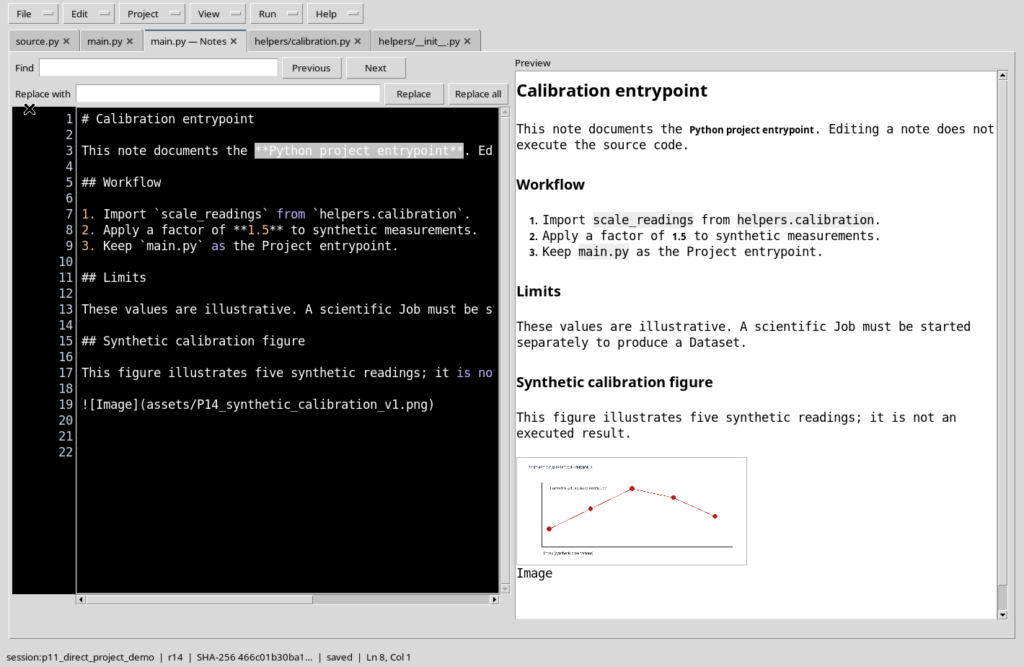
In the Source view of the note, select a word or phrase and choose Note format → Bold. The editor adds the ** delimiters around the selection: for example **Python project entrypoint**. In the Rendered preview panel the text appears in bold. The markup remains visible in Source and can be edited like normal text.
5. Italic and undoing changes
The Italic command uses single asterisks, for example *esempio*. To undo a formatting, use Undo on the Markdown document and check Source again. In some cases the two delimiters of a selection are inserted as separate editing operations: a single Undo may not completely restore the phrase. Always check the resulting text before continuing.
6. Heading: creating a readable hierarchy
The Heading 1, Heading 2 and Heading 3 commands insert the corresponding Markdown levels, useful for structuring a technical report. For example, # Scopo identifies a main heading and ## Procedura a subsection. Avoid choosing a level just to get larger characters: the hierarchy also matters for Outline navigation.
7. Inline code and Code block
Inline code highlights short identifiers such as scale_readings or main.py. Code block instead delimits a fragment over several lines. In a scientific note these functions distinguish reproducible instructions from explanations. A code block inserted in the note is not executed: the Runner uses the real Python source.
8. Bulleted and numbered lists
Bullet list and Numbered list insert text templates for describing prerequisites and steps. A numbered sequence is suitable for a protocol; a bulleted list for assumptions and limits. The text remains in Markdown and can be reordered manually. After inserting, check the preview: an out-of-place empty line can break a list.
9. Tables, links, quotes and separators
The menu offers Insert table for a Markdown table with headers and rows; Insert link for a link; Insert quote for a quoted block and Insert rule for a separator line. The contents generated are templates to be completed and checked. Text color concerns the presentation of the document: it does not give the data numeric meaning or measurement quality.
10. Minimal example of a technical note
The following fragment is an example of documentation to insert in the Source view, not a script to run.
# Calibration notes

## Input
- Five synthetic temperature readings.
- One illustrative calibration figure.

## Interpretation
**Illustrative only:** these values are not a published result.
The Python entrypoint is `main.py`.
In Rendered preview, check the structure before publishing.
11. Document changes and Save
The Notes tab signals changes not yet saved. File → Save registers the note in the authorised context; it is not the same as saving or launching main.py. It is prudent to save before starting to manage images, to distinguish formatting changes from changes to the resources.
12. Why attach a PNG figure
A figure can illustrate a diagram, a calibration curve, a micrograph or the layout of an experiment. The test uses a synthetic plot, with five observations, prepared as a PNG file. The image serves only to explain the procedure; it is not a computation output of the Workspace and does not replace a scientific Dataset with units and provenance.
13. The commands of the Note images menu
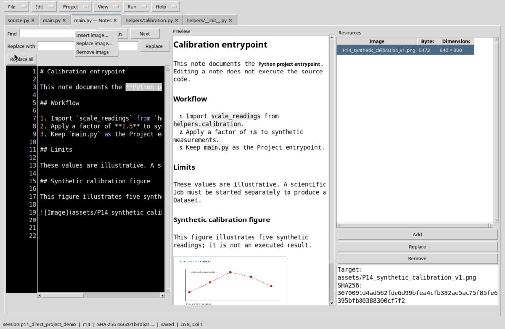
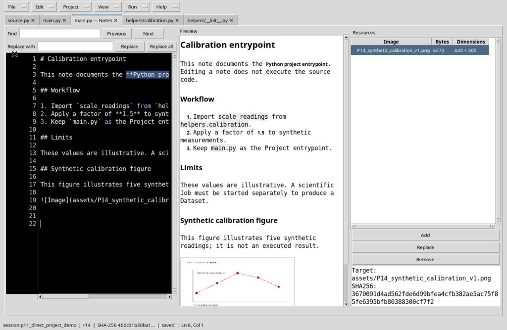
With the note active, open Edit → Note images: the entries available are Insert image…, Replace image… and Remove image. The same main operations can be reached from the Resources panel with the Add, Replace and Remove buttons. The availability of the entries depends on the document, the permissions and the presence of selectable resources.
14. Inserting a PNG file into the note
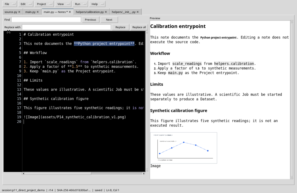
Place the cursor at the desired point in the text and choose Note images → Insert image…. The original file chooser filters PNG files. Select a compatible local image and confirm with Open. The editor acquires a managed resource: it does not simply insert the absolute path of the file, which would not be portable.
15. Limits of managed resources
In the version considered the image must be a valid PNG, no larger than 4 MiB, with width and height between 1 and 4096 pixels. A document can have at most 32 items and a total managed size not exceeding 16 MiB. The logical name must have a portable format. These limits are input constraints, not criteria for the scientific quality of the image.
16. The reference inserted in the Markdown
After Insert image… the Source view contains a reference similar to this:
The assets/ part indicates a resource managed by the document, not a directory to be created manually. The actual name derives from the chosen file or from the associated resource. Rendered preview displays the figure using the data registered in the editor.
17. Saving text and image together
After inserting, use File → Save. The note associates the text and the image with the persistent Markdown document. Check that the modification indicator disappears and that the plot is still visible in Rendered preview. The mere preview of a resource does not prove that the file has been saved.
18. Replacing an image without changing the link
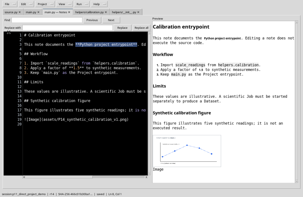
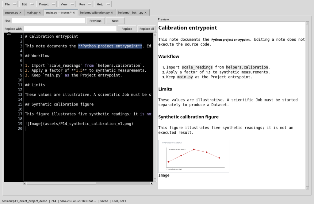
Open Note images → Replace image… after choosing the resource to replace in Resources. Select the new PNG and check the preview. In the example the blue plot is replaced by a red one: the logical name in the Markdown reference remains the same, but the binary data of the image change. A new Save is needed to make the replacement persistent.
19. Do not confuse name and content of the resource
A reference assets/nome.png identifies the logical resource of the document. After Replace image…, that name may continue to appear unchanged while the image shown is different. This is why it is important to check Rendered preview and, when needed, the information shown in Resources. A change to the image does not automatically mean that the scientific measurements have changed.
20. Adding a second temporary image
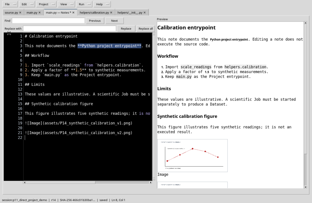
To understand removal, you can insert a second test PNG with Insert image… and select it in the list of resources. In the example it is an illustrative copy intended to be removed. It is useful to check the name before proceeding, especially when the images have very similar names.
21. Remove image does not automatically delete the Markdown
Select the resource and use Remove image. The operation removes it from the managed resources, but leaves in the text the Markdown reference that had been inserted. A reference left without a resource produces an unavailable figure in the preview. So look for the  line relating to that image, delete it manually and save the note.
22. Checking the Resources panel
Open View → Note panes and zoom → Resources. The table shows the name of the resource, the size in bytes and the resolution in pixels. Selecting a row shows details and the Add, Replace and Remove buttons. Keep this panel open while working on images; close it when you return to ordinary editing to save space in the source.
23. Checking version and association with Properties
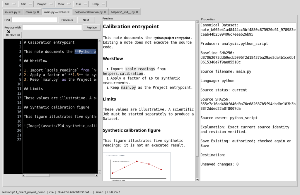
Open View → Note panes and zoom → Properties to examine the identity of the document, the associated source file and the state of the source. In the example Source filename: main.py and Source status: current appear. These are informative properties, not a direct editor of the source or of the scientific metadata. The identity check is repeated when saving.
24. The difference between Save and Publish New
Save updates the main document associated with the Python file, when the Session and the revision allow it. Publish New instead creates a distinct Markdown copy, with a new Dataset identifier; the primary document must not be replaced or reassigned automatically. It is a useful choice when you want to keep an independent version for consultation.
25. Opening Publish New and understanding the fields
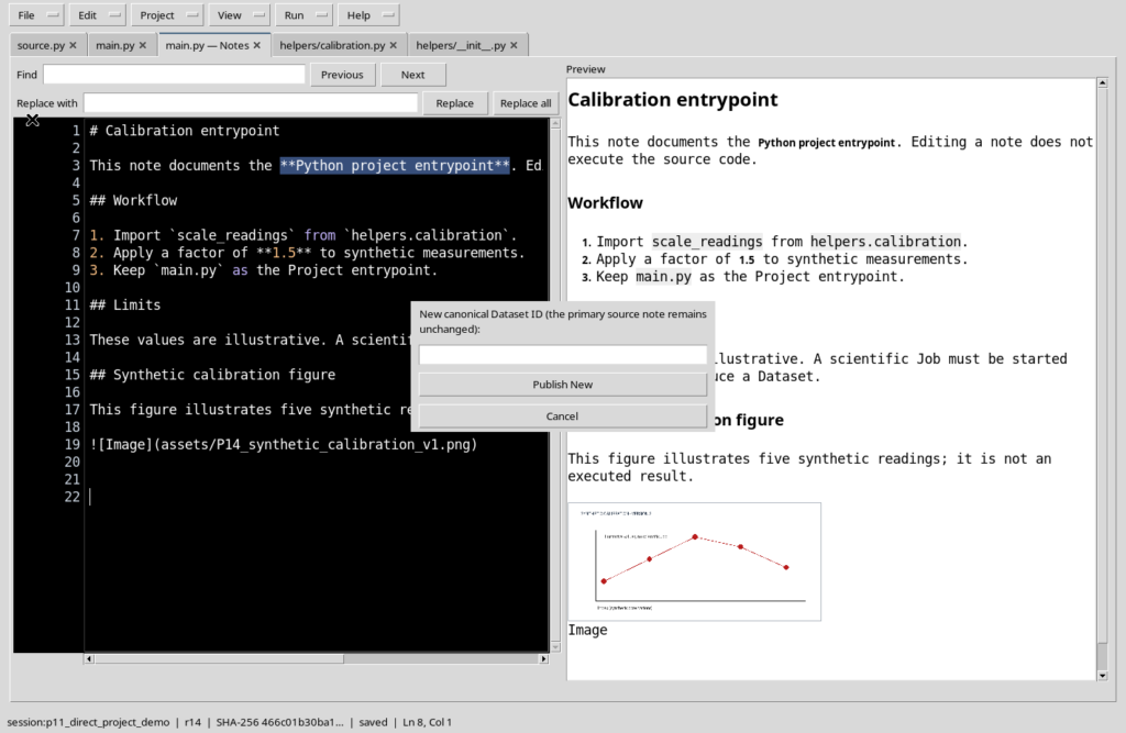
With Source active, the note shortcut Ctrl+Shift+S opens the Publish New document copy window. The field requires a new canonical identifier. The Publish New and Cancel buttons respectively create the copy and abandon the operation. Use a distinct and meaningful name, without confusing it with the identity of the main.py file.
26. Cancel and the copy actually published
If you choose Cancel, the window closes and the main note remains unchanged. If you confirm Publish New with a valid identifier, another Markdown document is created: the new Dataset does not replace the note linked to the source. In our example the copy also keeps the PNG resource present in the document. Publishing the copy is not the same as running a Job.
27. Checks before closing the note
Check that the document does not signal unsaved changes, that the preview contains no orphaned image references and that Properties shows the correct association with the source. Operations on notes require the relevant Session; a changed source or a document already modified elsewhere may lead to the save being refused. In that case keep the draft and check the correct version before trying again. Do not bypass the checks by resorting to internal functions.
28. Back to the Python code and summary
Use View → Show Notes to hide the note and recover the source editing area, preferably with the unnecessary side panels closed. The figures remain in the documentation already saved and the main.py file remains a normal Python source. The operations covered here did not require Script Library, Runner, Debugger or Jobs: the chapter concerns only the preparation and preservation of illustrated Markdown notes.