

Scientific calibration with the GX-TXT public APIs
With Octave Script Workspace a GNU Octave script can use scientific data already registered in the Session and publish a new Dataset without directly accessing the storage files. In this example we will read five synthetic voltages, apply a double gain chosen in the Runner and keep the corrected values through the GX-TXT public APIs.
The procedures refer to GX-TXT DEV112-P005, module Octave Script Workspace 1.8.3. The GUI labels are given in English and the code contains English comments. The editor uses the actual High Contrast Dark theme; the other controls keep the native Tk/ttk look.
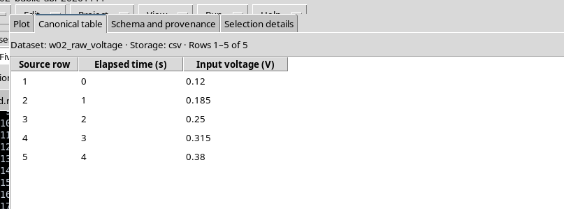
1. The Scientific Problem and the Five Starting Data
Suppose we have five voltage readings, in volts, acquired at successive times. The chosen gain is dimensionless and equal to 1.6. The relation used is:
V_corrected = gain × V_input
The input Dataset must have been previously published in the Session with the table.generic contract and with the stable variable IDs time_s and voltage_V. To prepare it you can follow the guide «Publishing numerical results and text output», adapting values and identifiers.
| Time (s) | Initial voltage (V) |
|---|---|
| 0 | 0.120 |
| 1 | 0.185 |
| 2 | 0.250 |
| 3 | 0.315 |
| 4 | 0.380 |
These data are entirely synthetic and do not come from an instrument.
2. Creating a Session Script and Declaring the Required APIs
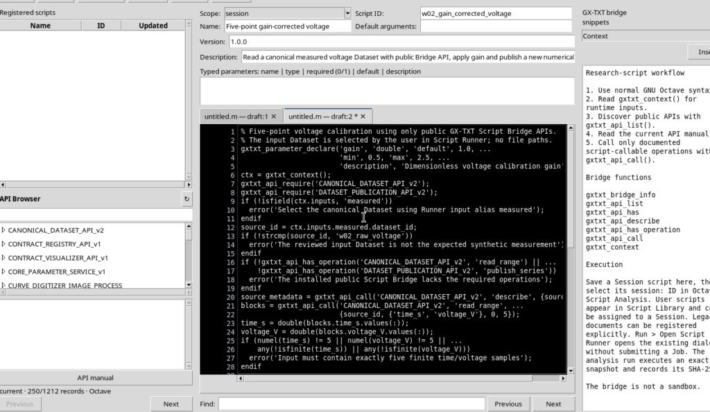
Open Octave Script Workspace, choose File → New Script and keep Scope: session. Assign an identifier, for example w02_gain_corrected_voltage, a name and a description; then save with File → Save.
In the Required APIs field enter exactly the two public APIs, separated by a semicolon:
CANONICAL_DATASET_API_v2;DATASET_PUBLICATION_API_v2The first provides canonical access to the data, the second handles numerical publication. Declaring them lets the Runner check their availability before the computation.
3. Complete GNU Octave Script
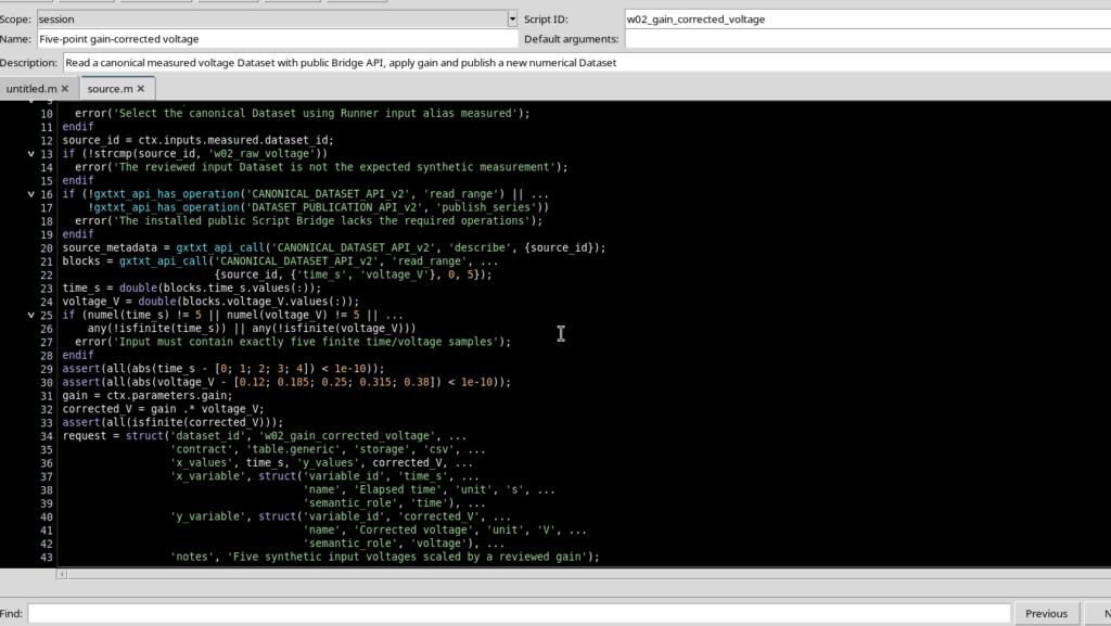
The program uses the GX-TXT public Bridge, without opening local files or using private framework commands. Copy the code into the editor; the comments are in English.
% Five-point voltage calibration using only public GX-TXT Script Bridge APIs.
% The input Dataset is selected by the user in Script Runner; no file paths.
gxtxt_parameter_declare('gain', 'double', 'default', 1.0, ...
                        'min', 0.5, 'max', 2.5, ...
                        'description', 'Dimensionless voltage calibration gain');
ctx = gxtxt_context();
gxtxt_api_require('CANONICAL_DATASET_API_v2');
gxtxt_api_require('DATASET_PUBLICATION_API_v2');
if (!isfield(ctx.inputs, 'measured'))
  error('Select the canonical Dataset using Runner input alias measured');
endif
source_id = ctx.inputs.measured.dataset_id;
if (!strcmp(source_id, 'w02_raw_voltage'))
  error('The reviewed input Dataset is not the expected synthetic measurement');
endif
if (!gxtxt_api_has_operation('CANONICAL_DATASET_API_v2', 'read_range') || ...
    !gxtxt_api_has_operation('DATASET_PUBLICATION_API_v2', 'publish_series'))
  error('The installed public Script Bridge lacks the required operations');
endif
source_metadata = gxtxt_api_call('CANONICAL_DATASET_API_v2', 'describe', {source_id});
blocks = gxtxt_api_call('CANONICAL_DATASET_API_v2', 'read_range', ...
                        {source_id, {'time_s', 'voltage_V'}, 0, 5});
time_s = double(blocks.time_s.values(:));
voltage_V = double(blocks.voltage_V.values(:));
if (numel(time_s) != 5 || numel(voltage_V) != 5 || ...
    any(!isfinite(time_s)) || any(!isfinite(voltage_V)))
  error('Input must contain exactly five finite time/voltage samples');
endif
assert(all(abs(time_s - [0; 1; 2; 3; 4]) < 1e-10));
assert(all(abs(voltage_V - [0.12; 0.185; 0.25; 0.315; 0.38]) < 1e-10));
gain = ctx.parameters.gain;
corrected_V = gain .* voltage_V;
assert(all(isfinite(corrected_V)));
request = struct('dataset_id', 'w02_gain_corrected_voltage', ...
                 'contract', 'table.generic', 'storage', 'csv', ...
                 'x_values', time_s, 'y_values', corrected_V, ...
                 'x_variable', struct('variable_id', 'time_s', ...
                                      'name', 'Elapsed time', 'unit', 's', ...
                                      'semantic_role', 'time'), ...
                 'y_variable', struct('variable_id', 'corrected_V', ...
                                      'name', 'Corrected voltage', 'unit', 'V', ...
                                      'semantic_role', 'voltage'), ...
                 'notes', 'Five synthetic input voltages scaled by a reviewed gain');
request.source_dataset_ids = {source_id};
request.source_variable_ids = {'time_s', 'voltage_V'};
request.source = source_id;
request.provenance = 'Gain-adjusted synthetic voltage from verified canonical input';
published = gxtxt_api_call('DATASET_PUBLICATION_API_v2', 'publish_series', {request});
fprintf('W02_INPUT_DATASET=%s\n', source_id);
fprintf('W02_GAIN=%.2f\n', gain);
fprintf('W02_POINT_COUNT=%d\n', numel(time_s));
for k = 1:numel(time_s)
  fprintf('W02_ROW=%d t=%.1f raw=%.3f corrected=%.3f\n', ...
          k, time_s(k), voltage_V(k), corrected_V(k));
endfor
disp('W02_PUBLICATION_COMPLETE');
disp(published);
In the first part the script checks the selected Dataset, the availability of the APIs and the numerical content. In the second part it computes the result, publishes it and prints a five-line summary. The identifiers used in the code must match those actually registered in the Session.
4. The Declared Parameter and the Execution Context
gxtxt_parameter_declare declares a parameter called gain, of type double, with default value 1.0, minimum 0.5 and maximum 2.5. The declaration is recognized when the source is registered; it does not start a Job.
gxtxt_context() returns the context of the specific execution. From ctx.parameters.gain you get the value validated by the user; from ctx.inputs.measured.dataset_id you get the identifier of the Dataset bound to the semantic alias measured.
The script must not build the physical path of the Dataset: the Runner provides a logical reference, checked in the current Session.
5. Discovering the Public Operations and Reading the Data
gxtxt_api_require requires the two APIs before proceeding. With gxtxt_api_has_operation you check that precisely the read_range and publish_series operations are available. A missing operation produces a recognizable error, not an empty result to be interpreted arbitrarily.
The general function gxtxt_api_call(api_id, operation, args) sends a call to a registered public service. The arguments of each operation are passed in an Octave cell array; the target API determines the accepted types and the structure of the result.
The describe command returns the metadata of the selected Dataset. To read the five values you use:
blocks = gxtxt_api_call('CANONICAL_DATASET_API_v2', 'read_range', ...
                        {source_id, {'time_s', 'voltage_V'}, 0, 5});
time_s = double(blocks.time_s.values(:));
voltage_V = double(blocks.voltage_V.values(:));
The range starts from row 0 (zero-based index) and requests 5 samples. The answer is a structure indexed by the stable variable IDs; the individual blocks contain typed values and read metadata. The .values(:) operation turns the numerical data into the column vectors used by Octave.
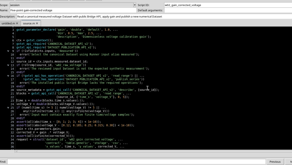
The assert statements check the five values of this exercise: for real experimental measurements, the criteria must be adapted to the actual Dataset.
6. Opening Script Runner and Choosing the Gain
After saving the source, use Run → Open Script Runner…. The Runner shows the script, the required APIs and the typed parameter gain (double) with initial value 1.0.
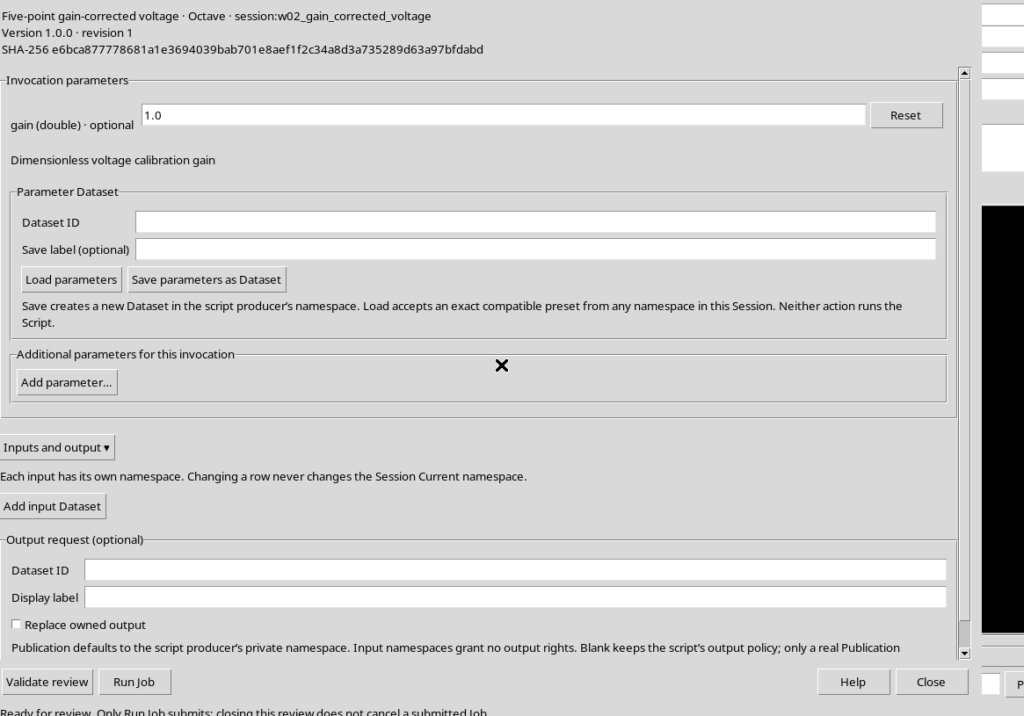
Set gain = 1.6. This change concerns the single scientific invocation and does not alter the source revision in the Registry.
7. Binding the measured Input and Identifying the Output
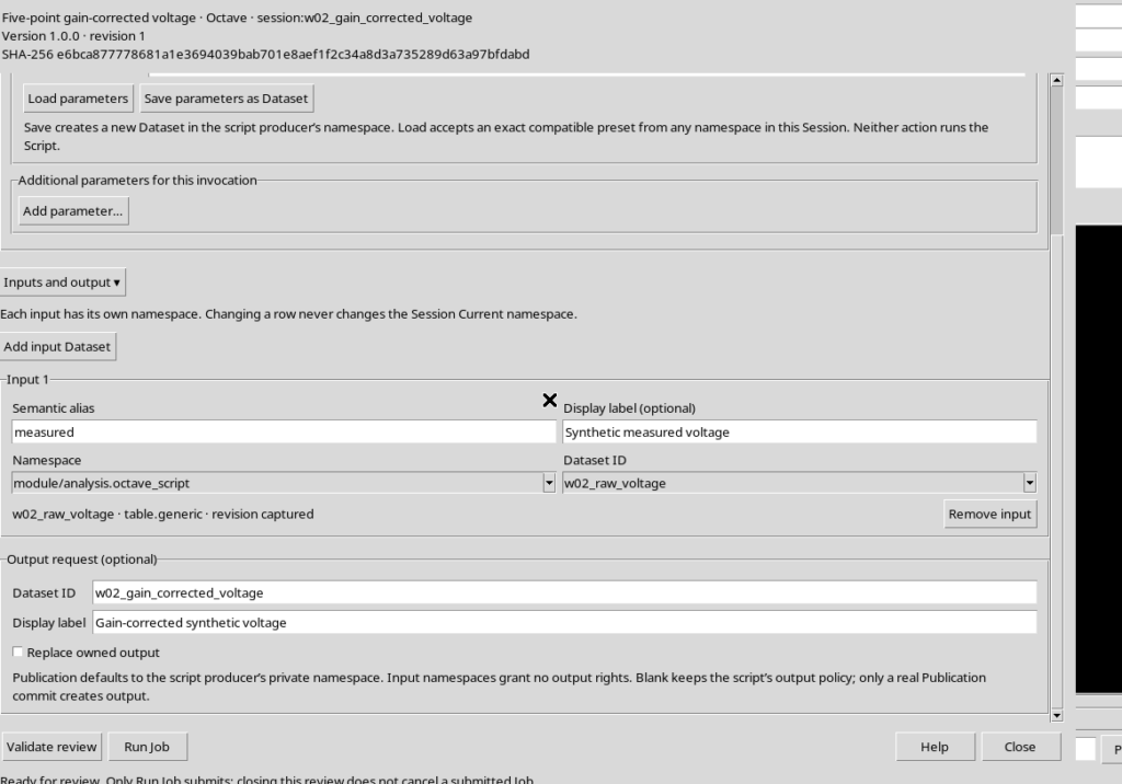
Open Inputs and output and choose Add input Dataset. Configure the three controls:
- Semantic alias: measured
- Namespace: module/analysis.octave_script
- Dataset ID: w02_raw_voltage
The Namespace is not a decorative detail. The Dataset used in the example belongs to the space of the producer module, so it might not appear if you choose base.
In the Output request (optional) section enter Dataset ID: w02_gain_corrected_voltage, add a descriptive label and leave Replace owned output unchecked. Filling in the field alone does not publish any result.
8. Validating the Request Without Running It
Press Validate review. With alias, input revision, APIs and parameter consistent, the Runner answers:
Review valid. No Job submitted; Run Job performs fresh admission checks.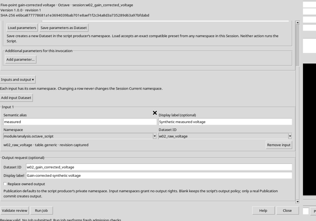
The revision of the input Dataset is recorded in the request. The check serves to prevent an unexpected replacement of the input from going unnoticed between the choice of data and the execution.
9. Starting GNU Octave and Examining the Job State
Press Run Job only once. GX-TXT runs the registered revision of the script, providing it with the measured alias and gain = 1.6.
In Run → Script Jobs Manager… the Job becomes COMPLETED after the computation. In case of FAILED, consult the Job details before attempting a new execution.
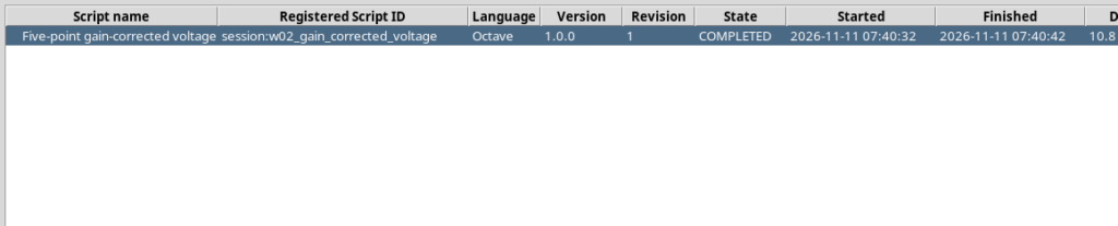
A Job keeps the executed revision, its own state and the output streams: it must not be confused with a published Dataset.
10. Reading the Results from Program Output
Choose Jobs → Open execution details, then Program output. The main lines actually produced by the script are:
W02_INPUT_DATASET=w02_raw_voltage
W02_GAIN=1.60
W02_POINT_COUNT=5
W02_ROW=1 t=0.0 raw=0.120 corrected=0.192
W02_ROW=2 t=1.0 raw=0.185 corrected=0.296
W02_ROW=3 t=2.0 raw=0.250 corrected=0.400
W02_ROW=4 t=3.0 raw=0.315 corrected=0.504
W02_ROW=5 t=4.0 raw=0.380 corrected=0.608
W02_PUBLICATION_COMPLETE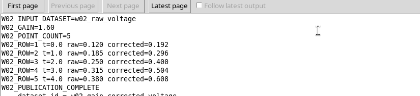
This text is an account of the execution. Numerical publication requires a separate call to the APIs: writing numbers to stdout is not enough to create a canonical Dataset.
11. Publishing a New Numerical Series
The script prepares a request structure containing dataset_id, contract: table.generic, storage: csv, the x_values and y_values vectors and the variable descriptors.
The actual publication operation is:
published = gxtxt_api_call('DATASET_PUBLICATION_API_v2', ...
                           'publish_series', {request});
Two output variables are declared: time_s with unit s and corrected_V with unit V. The request also records source_dataset_ids and source_variable_ids, so that the new Dataset keeps an explicit relationship with the original values.
The new Dataset is distinct from the input. The initial values are not modified, and no files or internal Registry entries are written by hand.
12. Comparing the Canonical Output Table with the Input
The published Dataset w02_gain_corrected_voltage uses table.generic and the CSV format. The Canonical table view tab shows five rows with time and corrected voltage.
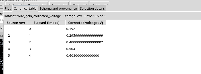
| Time (s) | Input (V) | Gain | Output (V) |
|---|---|---|---|
| 0 | 0.120 | 1.6 | 0.192 |
| 1 | 0.185 | 1.6 | 0.296 |
| 2 | 0.250 | 1.6 | 0.400 |
| 3 | 0.315 | 1.6 | 0.504 |
| 4 | 0.380 | 1.6 | 0.608 |
When displaying float64 numbers, representations such as 0.29599999999999999 may appear instead of 0.296. These are differences in binary representation, not new measurements: comparisons are made with an appropriate tolerance.
13. Checking Schema and Scientific Provenance
The Schema and provenance tab describes the published variables, including type, unit of measurement and semantic role. For this example time_s is a coordinate in seconds and corrected_V represents voltage data in volts.
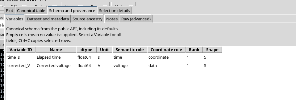
The provenance records w02_raw_voltage as source Dataset, time_s and voltage_V as starting variables and analysis.octave_script as producer of the new result. This information documents the link between two Datasets without falsely attributing an instrumental origin to the synthetic data.
14. Common Problems and Summary
If the Dataset does not appear in Add input Dataset, check the Namespace, the active Session and the identifier. If the script reports a missing input, check that the Semantic alias is exactly measured. If Validate review rejects the gain, check the double type and the declaration limits.
In case of an error during execution consult Program stderr and Diagnostic log. If the identifier of the output Dataset already exists, do not assume that the new invocation is allowed to overwrite it: a new result must be published with an available identity or with an explicitly authorized replacement procedure.
The complete workflow links canonical Dataset → Runner input → typed parameter → read_range → Octave computation → publish_series → new canonical Dataset. Using the public APIs separates the scientific computation from the physical details of storage and lets you check identity, revisions and provenance of the results.